Table of contents
Abstract......................................................................................................................................................................................... i
1. Introduction............................................................................................................................................................................ 1
2. Tracker................................................................................................................................................................................... 4
2.1 Transit Data...................................................................................................................................................................... 4
2.2 Translating Tri-Met terms into TCIP............................................................................................................................ 6
2.3 Transit AVL...................................................................................................................................................................... 7
2.4 Tracking and Trip Assignment...................................................................................................................................... 9
2.4.1 Generation of Candidate Trips........................................................................................................................ 11
2.4.2 Selection of Trip.................................................................................................................................................. 12
3. Filter...................................................................................................................................................................................... 16
3.1 Design............................................................................................................................................................................. 16
3.2 Determination of filter parameters............................................................................................................................... 21
4. Predictor............................................................................................................................................................................... 23
5. Examples............................................................................................................................................................................... 25
5.1 Example 1......................................................................................................................................................................... 25
5.2 Example 2......................................................................................................................................................................... 28
5.3 Example 3......................................................................................................................................................................... 29
6. Tri-Met Data Analysis........................................................................................................................................................ 30
6.1 State Plane Coordinates................................................................................................................................................ 30
6.2 Sample Sizes and Rates................................................................................................................................................. 31
6.3 Trip Assignment............................................................................................................................................................ 34
6.4 Deviation......................................................................................................................................................................... 37
7. Prediction in Adverse Conditions.................................................................................................................................... 43
7.1 Schedule Adherence..................................................................................................................................................... 44
7.2 Prediction........................................................................................................................................................................ 45
7.3 Modified Prediction - The Value of a Bridge
Open Signal...................................................................................... 48
8. Conclusions.......................................................................................................................................................................... 49
References................................................................................................................................................................................. 50
Appendix A: Searching a Geographic Data Set Using Tiles........................................................................................... 51
Appendix B: Distance Algorithm.......................................................................................................................................... 52
List of Figures
Figure 1.1: Overall design for a general prediction
system........................................................................ 3
Figure 2.1: A pattern with TPI’s and shape-points
identified..................................................................... 5
Figure 2.2: Vehicle locations in state-plane
coordinates............................................................................ 8
Figure 2.3: Distance from reported position to nearest
point on pattern...................................................... 8
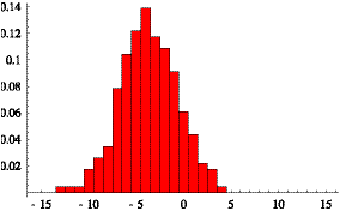
Figure 2.4 Time series of computed distance-into-trip............................................................................. 14
Figure 2.5: Time series of computed distance for a
block........................................................................ 14
Figure 2.6: Time series of distance from report to
nearest point on block................................................. 15
Figure 3.1: Time series of distance-into-trip........................................................................................... 20
Figure 3.2: Time series of estimated speed............................................................................................ 20
Figure 3.3: Residuals between measurements and
estimates................................................................... 20
Figure 5.1: Schedule based s(x, t) and solution trajectories...................................................................... 27
Figure 5.2: Contour plot of speed, darker is slower................................................................................. 27
Figure 5.3: Travel time as a function of departure time........................................................................... 28
Figure 5.3: Probability of correct predictions mad by
the schedule on the left
................. and the algorithm presented on the right............................................................................... 29
Figure 6.1: State-plane map of Portland bus routes................................................................................. 30
Figure 6.2: Reports from train 668......................................................................................................... 31
Figure 6.3: Distribution of the number of samples per
train on day 9/11/2000.
................. There are 8,473 samples..................................................................................................... 32
Figure 6.4: Trains with large sample sets on day
9/11/2000..................................................................... 32
Figure 6.5: Time between reports for train 668 on day
9/11/2000............................................................. 33
Figure 6.6: Time between reports for train 7240 on day
9/11/2000........................................................... 33
Figure 6.7: Time between reports for train 1706 on day
9/11/2000........................................................... 34
Figure 6.8: Time series of distance into trip for train
668 on day 9/11/2000............................................... 34
Figure 6.9: Time series of distance-into-trip for train
1724 on day 9/11/2000............................................. 35
Figure 6.10: Time series of distance-into-trip for train
1706 on day 9/11/2000........................................... 35
Figure 6.11: Train 668 gap in trip assignment......................................................................................... 36
Figure 6.12: Pattern for train 668.......................................................................................................... 37
Figure 6.13: Difference of reported and computed
deviation for train 7234 on day 9/11/2000..................... 38
Figure 6.14: Time series of distance-into-trip for train
7234 on day 9/11/2000........................................... 38
Figure 6.15: Difference of reported and computed
deviation for train 7003 on day 9/11/2000..................... 39
Figure 6.16: Comparison of reported and computed
deviation for train 7003
................. on
trip 10 on day 9/11/2000................................................................................................ 39
Figure 6.17: Superposition of samples of train 7003 on
trips 10 and 11 on day 9/11/2000........................... 40
Figure 6.18: Sample 59 for train 7003 is not on trip 11
on day 9/11/2000................................................... 40
Figure 6.19: Time series of distance-into-trip for train
7003 on trips 12 and 13 on day 9/11/2000................ 41
Figure 6.20: Prediction error as a function of time
before arrival............................................................. 42
Figure 7.1: Hawthorne Bridge location on multiple blocks
of scheduled transit work................................. 43
Figure 7.2: Example train 688 over the course of
11/13/2000. Vertical bars are
................. periods when the bridge is open........................................................................................... 45
Figure 7.3: Magnified version of the fifteenth trip of
train 668 that is impacted by the
................. bridge opening at minute 1116 (6:36 PM).............................................................................. 46
Figure 7.4: Fast update rate data suitable for use with
a Kalman filter predictor....................................... 46
Figure 7.5: Probability of correctly predicting the
vehicle arrival downstream
................. of the bridge for all bridge crossings identified....................................................................... 47
Figure 7.6: Probability density for correct prediction
for trips impacted by a bridge opening...................... 47
Figure 7.7: Prediction made assuming real-time bridge
opening data is available....................................... 48
Figure A.1: A point on a tile.................................................................................................................. 51
Figure B.1: Distance from point to line segment..................................................................................... 52
This report documents the activities undertaken by the University
of Washington as part of a contract supported by TransNow and Tri-Met through
Portland State University. In this report, we present three major ideas.
First, we document the performance of a previously published
prediction algorithm [1] appropriate for use with Tri-Met’s scheduling and
Automatic Vehicle Location (AVL) system. This algorithm provides a clearly
defined open and independent mechanism to assign vehicles to trips and predict
arrival/departure times. The algorithm provides open and detailed assignment
and prediction algorithms.
Secondly, we present data reduction and analysis for a week
of data provided by Tri-Met. This effort documents the significant improvement
in passenger information over the schedule available by using real-time information.
It also identifies anomalies in the data stream that may cause trip assignment
and prediction algorithms to produce erroneous information. We compare the
results of the algorithms presented with deviation estimates provided in the
Tri-Met data and argue that the algorithm handles exceptions more correctly
than the process that created the deviation for comparison.
Thirdly, we examine the performance of the algorithm under
adverse conditions. The adverse condition available for testing is the unscheduled
opening of the Hawthorne Bridge in Portland, Oregon. Data from the bridge
opening log book for the month of November 2000 were used with matching
schedule and AVL data to test the efficacy of the algorithm. Further, we
quantify the improvement possible if additional information from a sensor on
the bridge indicating its status as
open or closed was available.
In addition to the demonstration of the prediction efficacy,
the report documents a methodology to perform data fusion in making
predictions. This data fusion can incorporate information beyond the schedule.
This may include traffic, weather, or historical information.
We present a general structure for creating a system that
can take vehicle location data as input and produce predictions of arrival or
departure at subsequent points along a planned route. This general structure
has been developed over a number of years and reported in several manuscripts
[2, 3, 4]. It has been implemented in the form of an application called
MyBus.org [5] using the AVL system operated by the transit carrier Metro in
King County, Washington.
The specific task covered in this report is the reuse of
this general structure with schedule and vehicle data from the Tri-Met Transit
system in Portland, Oregon, to demonstrate that the concepts used in the
overall design generalize to a transit system using different technologies for
positioning and scheduling.
We make three assumptions in solving the general problem of
predicting arrival or departure of transit vehicles: (1) there is a fleet of
transit vehicles that travel along prescribed routes, (2) there is a “transit
database” that defines the schedule times and the geographical layout of every
route and time point, and (3) there is an automatic vehicle location (AVL) system,
where each vehicle in the fleet is equipped with a transmitter and periodically
reports its progress back to a transit management center.
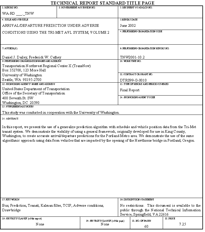
Figure 1.1 is a data flow diagram for the general problem.
The details of the definition of the variables shown in the figure will become
clear in subsequent sections. There are three important components in this
design, as shown in Figure 1.1. The operation of the generalized algorithm is
illustrated by following the data as it flows through these three components.
The GPS data from the vehicles is combined with spatial and temporal schedule
information in the first component, the “Tracker,” to produce an assignment of
a vehicle to the task scheduled by the transit operator. Next, the data pass
through the second component, a “Filter,” that is an implementation of a Kalman
filter process to make optimal estimates of the location and the speed of the
vehicle. The Filter also generates a continuous stream of data that is updated
at pre-selected temporal intervals. These data are then used in the third
component, a “Predictor,” that generates the time of arrival or departure at a
variety of downstream locations for each vehicle observed. This report details
the data and functionality of each of these components.
Figure 1.1: Overall design for a general prediction
system.
The first component of the algorithm is the Tracker. It
assigns each observed vehicle to the activity which that vehicle is scheduled
to perform. Both spatial and temporal schedule data from a transit property are
necessary for this task. It has been our observation that the schedule data are
represented differently in each transit property. One goal of this effort is to
demonstrate that our framework will generalize. This generalization is in part
possible because of the reliance on a generic set of definitions for the data
that make up the temporal and spatial schedule information. This set of generic
definitions is taken from the Transit Communications Interface Profiles (TCIP)
Framework [6]. We first describe the TCIP data necessary to accomplish the task
of the Tracker. We then discuss the mapping between Tri-Met’s representation of
the data and the TCIP representation. We present the AVL data framework being
used. Finally, we present the tracking and trip assignment algorithm.
To clarify the terminology used here, we present a
conceptual description of five relevant database elements in TCIP terms: (1)
time-point, (2) time-point-interval (TPI), (3) pattern, (4) trip, and (5)
block.
A time-point is a
named location. The location is generally defined by two coordinates, either
Cartesian state-plane coordinates or geodetic latitude and longitude. For the
purposes of this report, we assume NAD-83 state-plane coordinates and also
assume that the transformation from geodetic to state-plane coordinates, and
its inverse, are known [7]. We choose to use Cartesian coordinates for
computational reasons as the geometry and metric are Euclidean rather that
ellipsoidal. The time-points are the locations at which the transit vehicles
are scheduled to arrive or depart.
A time-point-interval
(TPI) is a polygonal path representing a stretch of road directed from one
time-point to another. The path is geographically defined by a list of
“shape-points,” where a shape-point is simply an unnamed location. Since one
frequently needs to determine the distance of a vehicle along a path, each
shape-point is augmented with its own distance-into-path. The length of a TPI
is the distance into path of the last shape-point (the ending time-point).
A pattern is a
“route” made up of a sequence of TPI’s, where the ending time-point of the ith TPI is the starting
time-point of the (i+1)th. Note that the sequence of
TPI’s on a pattern determines a sequence of time-points on the pattern. (The
converse is not necessarily true since there may be more that one TPI running
from one time-point to another.) The distance-into-pattern of a TPI is defined
to be the sum of the lengths of the preceding TPI’s and the length of a pattern
is the sum of the lengths of its TPI’s. For a vehicle traversing a pattern, the
index of the TPI that the vehicle is on and the vehicle’s distance-into-TPI
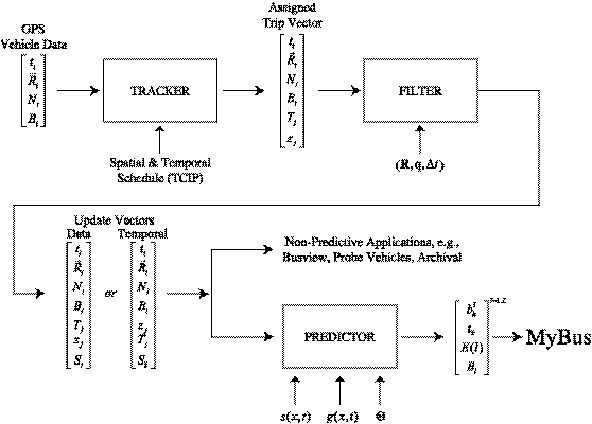
uniquely determine the distance-into-pattern of the vehicle. Figure 2.1 shows a
sample pattern plotted in state-plane coordinates, with origin translated
to the corner of Salmon and 5th.
Figure 2.1: A pattern with TPI’s and shape-points
identified.
A trip, labeled Tj in Figure 1.1,
is an assignment of schedule times to time-points on a pattern. More precisely,
a trip specifies a start time and end time for every TPI on the pattern in such
a way that the end time for the ith
TPI is no greater than the start time for the (i+1)th. Note
that it is possible for the same time-point to be assigned two successive
times, in which case we say that a layover
is scheduled at that point. Note also that a trip specifies a travel time for
each of its TPI’s, and different trips on the same TPI may specify different
travel times depending on the time of day. The set of all trips is partitioned
into blocks, as defined below.
A block, labeled bi in Figure 1.1, is a
sequence of trips such that the schedule time for the end of the ith trip is no greater than
the schedule time for the start of the (i+1)th trip. If the end
time-point of the ith trip
is the same as the start time-point for the (i+1)th, but
the schedule times are different, then, as in the preceding paragraph, we say
that a layover is scheduled at that point. Each transit vehicle is assigned a
block to follow over the course of the day. Some blocks are long and are
covered by different vehicles at different times of the day.
The basic conceptual components from TCIP and those from the
Tri-Met schedule differ slightly. The main difference between the two systems
is in the definition of a bus route, which is represented in the Tri-Met system
by a “link” rather than a pattern, as in the TCIP system. The basic Tri-Met
concepts are: (1) location, (2) link, (3) trip, and (4) train; whereas the TCIP
abstractions are: (1) time point, (2) time-point-interval, (3) pattern, (4)
trip, and (5) block.
A location is
specified by a name, latitude, and longitude. There are two types of location:
time-point and bus-stop.
A link consists
of two things: a polygonal path representing a bus route and a list of
locations consisting of time-points and bus-stops along the route. As in the
case of a TPI, the path is geographically defined by a list of shape-points. To
facilitate computation, each shape-point and location is augmented with its own
distance-into-path.
A trip is an
assignment of schedule times to time-point locations on a particular link. As
with the corresponding TCIP concept, the set of trips is partitioned into
blocks.
A train is
defined as a sequence of trips; this is a block in the TCIP case above.
As indicated in the preceding section, a preliminary step in
working with locations and shape-points is to transform their geodetic
coordinates to Cartesian coordinates. For this purpose, we used the Lambert
projection from the geodetic system to the NAD-83 Oregon North state plane
system.
Except for the notion of TPI, there is a clear
correspondence between Tri-Met and TCIP concepts. We use a simple process that
maps Tri-Met’s link data to TCIP TPI’s and associates a unique pattern to every
link. To do this, a link is traversed from beginning to end. For each pair of
successive time-point locations on the link, we define a TPI that connects the
first to the second. The shape-point list for this TPI consists of the two
time-points as well as the sub-sequence of link shape-points that lie between
the time-points. We also augment each TPI shape-point with its own
distance-into-TPI. This process subdivides each link into a sequence of
contiguous TPI’s that make up a pattern in TCIP terms.
AVL systems produce real-time reports of vehicle location
based on technologies such as dead reckoning or satellite GPS position
measurements. In the case of the Tri-Met AVL system, each vehicle in the fleet
is equipped with a GPS receiver and a radio transmitter. The vehicles
periodically transmit location reports back to the transit center. These
reports include the following information:
·
vehicle-identifier: Ni
in Figure 1.1,
·
block-identifier:
Bi in Figure 1.1,
·
time: ti
in Figure 1.1,
·
latitude and longitude:  in Figure 1.1.
Applications that make use of AVL data require the
information in a more usable form. For example, a graphical application that
displays vehicle location or measures distance between the vehicle and
landmarks must transform the reported geodetic coordinates into Cartesian
planar coordinates with a minimum of distortion. We use the NAD-83 state-plane
transformations to do this and assume, henceforth, that each AVL report is
automatically augmented with position coordinates in the same state-plane
coordinate system used in the schedule database.
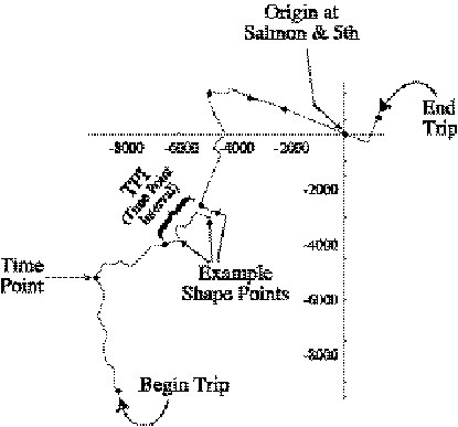
Figure 2.2 shows a state-plane plot of a sequence of vehicle
locations superimposed over a schedule pattern. In this figure, the coordinates
have been translated so that the origin is at the corner of Salmon and 5th. The
vehicle is moving towards the end of the pattern in the lower left quadrant.
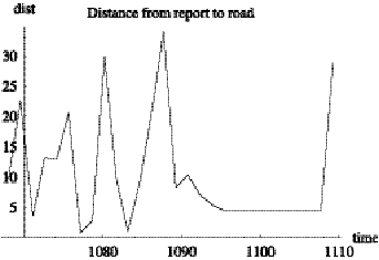
Figure 2.3 shows a corresponding time-series plot of distance (in feet) from
reported position to nearest point on pattern.
Figure 2.2:
Vehicle locations in state-plane coordinates.
Figure 2.3: Distance from reported position to nearest
point on pattern.
An application which computes schedule deviation or predicts
vehicle arrival times requires information in a form that is directly
correlated to the scheduled block of work. These data are the trip identifier
and the distance-into-trip, where distance-into-trip is defined to be the
distance along the underlying pattern. For example, if the vehicle
distance-into-trip equals that of a scheduled time-point, then schedule
deviation is just the difference of report time and schedule time.
Based on the definition of the data items, we assert that it
is straightforward to identify the vehicle location from the TCIP data pattern,
distance-into-pattern. That is, given trip and distance-into-trip, we can
determine block and state-plane location coordinates. The preceding definition
of trip requires that every trip is associated with a unique block, and the
pair (trip, distance-into-trip) determines the pair (pattern,
distance-into-pattern) exactly. The pair (pattern, distance-into-pattern)
uniquely determines both TPI and distance-into-TPI. By moving the appropriate
distance along the sequence of shape points on the identified TPI, we determine
a pair of successive shape points on either side of the vehicle. Finally, we
determine vehicle state-plane coordinates by interpolating between these two
shape-points.
The mapping from the tuple (block, time, vehicle location in
state-plane coordinates) is not as straightforward. In the next section, we
describe a procedure to determine trip and distance-into-trip given the block,
time, and vehicle location in state-plane coordinates.
Mapping AVL data to an assigned piece of scheduled work is
not straightforward. Vehicles may traverse the same pattern several times,
perhaps in different directions; in addition, they may be delayed or ahead of
schedule. As a result, there are ambiguities when assigning AVL reports to
trips. For example, if a vehicle is operating on a block that travels back and
forth over the same roadways between two destinations, and the vehicle is late
on a trip traveling one way, its position can be such that it could be
identified as late or it might be identified as early on the next trip,
traveling the other way. This sort of ambiguity is the reason that a
sophisticated tracker is needed.
We present a tracking methodology that determines trip and
distance-into-trip for transit vehicles that provide AVL reports. The basic
idea is to maintain a track on each vehicle which records the last report, trip
assignment, distance-into-trip, and other useful information. Tracks are then
updated as new reports are received. The trip assignment logic and
distance-into-trip calculation take advantage of previous track values in order
to improve efficiency, eliminate ambiguities, and increase probability of
update correctness.
The goal of the Tracker is to use an AVL report to produce a
track that contains the following
information:
·
vehicle-identifier Ni,
·
last associated AVL report  ,
,
·
trip Tj,
·
distance-into-trip zi,
·
TPI,
·
distance-into-TPI di,
·
deviation  ,
,
·
validity (true or false),
·
number of rejected updates,
where 1) the validity field
indicates whether or not the trip data can be used in subsequent processing, 2)
(TPI, distance-into-TPI) can be computed from (trip, distance-into-trip), and
3) deviation is defined to be the difference between the report time and
the interpolated schedule time for the distance-into-TPI of this report. The
interpolated schedule time
is defined to be the difference between the report time and
the interpolated schedule time for the distance-into-TPI of this report. The
interpolated schedule time  needed for this is
the starting time, t0 for
the TPI plus the time to traverse the distance-into-TPI, di, portion of the TPI at a known speed (s). The deviation,
needed for this is
the starting time, t0 for
the TPI plus the time to traverse the distance-into-TPI, di, portion of the TPI at a known speed (s). The deviation,
provides a temporal sanity check for
AVL reports.
The validity field of each track is initially marked invalid
and remains so until a report is received from which we can compute reasonable
trip data. A valid track will be marked invalid if the time since the last
report exceeds a specified duration or the number of rejected updates exceeds a
specified limit. An update is rejected if no trip data can be computed that are
reasonable with respect to the track data. This may be due to GPS measurement
error in the report or to previously accrued error in the track.
The essence of the tracking algorithm is based on the
classic paradigm of “generate and test” [8]. The rationale behind this approach
is that typically there are several feasible trip assignments for a report, and
we must test for the most likely one. For example, in the middle of a TPI a
single candidate will normally be determined; however, at the end of a TPI
there will be two or more, and near the end of a trip there may be four or more
candidates to choose from. The generate and test logic is the following:
1. Look
up the track with matching vehicle-identification, and if none are found, we
create a new track and mark it invalid.
2. Generate
a set of candidate trip data tuples (trip, distance-into-trip, TPI,
distance-into-TPI, deviation).
3. Apply
selection/test rules to determine the most likely choice.
4. Update
the track accordingly.
5. The
generation of candidate trips and trip selection rules are detailed below.
Generating candidate trips involves reasoning in both space
and time. When an AVL report is received, the candidate trips are established
using geographical and temporal proximity. The generate and test paradigm
requires a set of hypotheses from which the “correct” one is selected. In our
case, identifying candidate trips is equivalent to generating hypotheses. The
algorithm below identifies the candidates, and the algorithm in the next
section acts to select the correct one from the candidates.
The algorithm to identify the candidate trips is as follows:
1. Obtain
an AVL report
2. Define
a circular neighborhood  around the reported
position
around the reported
position  where the radius
  bounds the maximum
expected measurement error.
bounds the maximum
expected measurement error.
3. Determine
the tile  containing the point
  .
.
We
use an original “Tiling” technique to provide keys for fast searching of TPI’s.
In building an implementation of our algorithm, it is necessary to create an
efficient mechanism for accessing subsets of the large map data set. As a
result, a new “tiling” methodology is used for creating a tree to access the
TPI’s. The details of this new technique can be found in Appendix A.
4. Determine
the “time-feasible” pairs (trip, TPI) associated with the tile.
Using
the reported block and time, select a set of pairs (trip, TPI) where the trip
is on the reported block, the TPI lies on the trip’s underlying pattern, the
TPI intersects  (the tile
  is inflated by radius
 ), and the pair is “time-feasible.” “Time-feasible” means
that the time of the report lies in a specified time-window containing the
schedule times for the starting and ending time-points for the TPI. For
example, in our results presented later, we specified a window whose lower
limit was 20 minutes earlier than the TPI start time and whose upper limit was
90 minutes later than the TPI end time. A simple search through the block is
used to determine the set of these “time-feasible pairs.” Moreover, if the
track associated with this report is valid, then the search begins with the
last (trip, TPI) pair, or, if the last distance-into-TPI is less than
), and the pair is “time-feasible.” “Time-feasible” means
that the time of the report lies in a specified time-window containing the
schedule times for the starting and ending time-points for the TPI. For
example, in our results presented later, we specified a window whose lower
limit was 20 minutes earlier than the TPI start time and whose upper limit was
90 minutes later than the TPI end time. A simple search through the block is
used to determine the set of these “time-feasible pairs.” Moreover, if the
track associated with this report is valid, then the search begins with the
last (trip, TPI) pair, or, if the last distance-into-TPI is less than  , with the preceding pair.
5. Determine
the set of “space-feasible” triples from the “time-feasible” set.
Using
the reported location  and the pairs just
determined, we perform geometric processing to compute a set of “space-feasible
triples (trip, TPI, p) where p is a point on the TPI. A triple is
“space-feasible” if p locally
minimizes distance from the TPI to the reported position p and this distance is less than
and the pairs just
determined, we perform geometric processing to compute a set of “space-feasible
triples (trip, TPI, p) where p is a point on the TPI. A triple is
“space-feasible” if p locally
minimizes distance from the TPI to the reported position p and this distance is less than  .
.
The
distance used in this optimization is the distance from a point to a line
segment and is described in detail in Appendix B.
To
perform this minimization, we proceed as follows. Let the TPI polygonal path be
defined by the sequence of shape points  and represent an
arbitrary point p on the path
parametrically as a pair (k, d) where k is a shape-point index and d
is distance along the line segment
and represent an
arbitrary point p on the path
parametrically as a pair (k, d) where k is a shape-point index and d
is distance along the line segment  .
.
Let
 denote the
subsequence of shape-points representing an intersection sub-path of TPI with
tile
denote the
subsequence of shape-points representing an intersection sub-path of TPI with
tile  . Compute the distance rk
from
. Compute the distance rk
from  to each successive
line segment
to each successive
line segment  on this sub-path and
for each k such that
on this sub-path and
for each k such that  is a local minimum.
Compute the distance d along the
segment that specifies the minimizing point p.
The distance-into-TPI for point p is
simply the sum d + dk where dk is the distance-into-TPI of the kth shape point.
is a local minimum.
Compute the distance d along the
segment that specifies the minimizing point p.
The distance-into-TPI for point p is
simply the sum d + dk where dk is the distance-into-TPI of the kth shape point.
We assert that the AVL report belongs to one of the
remaining trips that are “space-” and “time-feasible.”
In the last section we identified hypotheses or candidate
trips that need to be evaluated to determine the best estimate of the trip from
which the AVL report arises. In this section, we describe the rules and tests
that we apply when selecting a candidate-trip data tuple to update the track. The rules are a set of
conditionals.
If the candidate set is empty,
Then
no selection is possible.
In
this case, the vehicle track associated with this report will either be marked
invalid or its update rejection count will be incremented, as discussed
previously.
If the current report is associated
with an invalid track,
Then
select the candidate tuple whose deviation has minimum absolute value.
If the associated track is valid,
Then
we subject the set of candidates to some screening tests and eliminate any
candidate that fails a test.
For each candidate-trip data tuple, let
 denote the distance
traveled by the vehicle since the last report, assuming that both track and the
tuple represents the “truth” (i.e., the error in the candidate position
measurement is within the specified tolerance
denote the distance
traveled by the vehicle since the last report, assuming that both track and the
tuple represents the “truth” (i.e., the error in the candidate position
measurement is within the specified tolerance  ). Let
  denote the
corresponding change in time. We assume that any error in reported time is
insignificant in comparison to position error.
denote the
corresponding change in time. We assume that any error in reported time is
insignificant in comparison to position error.
1. The
first screening test corresponds to the reasonable assumption that the bus
moves forward along any pattern: an acceptable tuple must satisfy  .
.
2. The
second test checks for tuples such that  is reasonable given
the time step
is reasonable given
the time step  . We predict the maximum distance
  that the vehicle
could have traveled in time
that the vehicle
could have traveled in time  based on speed limit
and schedule data and require that
based on speed limit
and schedule data and require that  .
.
If the remaining set is empty,
Then
no selection is possible.
If only one candidate survives,
Then
it is selected,
If more than one candidate tuple
survives these tests,
Then
we apply preference rules.
If there are two candidates which
together indicate that the vehicle is on a layover between trips (that is, one
candidate indicates that vehicle is at the end of the track’s last trip and
another candidate indicates that it is at the start of the next trip on the
block)
Then, in this case, we select the
candidate whose deviation has minimum absolute value. (We effectively declare a
trip transition halfway through the layover.)
If the layover rule is not applicable,
Then we predict an expected distance  that the vehicle
would have traveled in time
that the vehicle
would have traveled in time  based on speed limit
and schedule data and select the candidate whose value for
based on speed limit
and schedule data and select the candidate whose value for  is closest to
  .
.
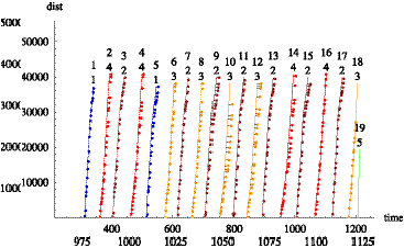
Figure 2.4 shows a time-series plot of computed
distance-into-trip for a specific vehicle on several trips. (Here, time is
measured in minutes after midnight and distance in feet.) Each continuous curve
rising from left to right corresponds to a trip and consists of a polygonal
line joining scheduled time-points. Each curve is labeled with two numbers. The
upper number identifies the trip, while the lower number identifies the trip’s
pattern. (Note that the trip’s pattern number repeats when the vehicle travels
over the same physical streets repeatedly.) The short horizontal line segments
are drawn to help visualize estimated schedule deviations of the vehicle. Figure
2.5 shows a similar plot for every trip on a block.
Figure 2.4 Time
series of computed distance-into-trip.
Figure 2.5: Time series of computed distance for a
block.
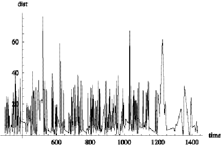
Figure 2.6 shows an example time-series plot of the distance from reported
position to nearest point on trip over an entire block.
Figure 2.6: Time series of distance from report to
nearest point on block.
We use a Kalman filter/smoother to transform a sequence of
AVL measurements into estimates of vehicle dynamical state, including vehicle
speed. In this section, we describe the measurement and process models used in
the filter framework. The models depend on several parameters, including the
variances for measurement and process noise. We estimated representative values
experimentally using the method of maximum marginal likelihood as specified in
[9] and described in Section 3.2 below.
Recall that in order to implement a Kalman filter, the
following must be specified:
·
a state-space,
·
a measurement model,
·
a state transition model,
·
an initialization procedure.
Once these items are specified, one
may employ any one of a number of implementations of the Kalman filter/smoother
equations, (see [9, 10, 11, or12]) to transform a sequence of measurements into
a sequence of vehicle state estimates.
To represent the instantaneous
dynamical state of a vehicle, we selected a 3-dimensional state space. We
denote a vehicle state vector by
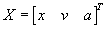 ,
,
where x is distance-into-pattern, v
is speed, and a is acceleration. (The
superscript T denotes transpose.) We
use the foot as unit of distance and minute as unit of time.
A measurement, z,
provided by the Tracker, is an estimate of the vehicle’s distance-into-trip,
and our measurement model is given by
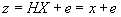 .
.
Here,  is the “measurement
matrix,” and e denotes a random
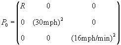
measurement error, assumed to have a Normal distribution with variance R. The variance is treated as a model
parameter with nominal value of R =
(500 ft)2. The value for R
was determined as described in Section 3.2.
is the “measurement
matrix,” and e denotes a random
measurement error, assumed to have a Normal distribution with variance R. The variance is treated as a model
parameter with nominal value of R =
(500 ft)2. The value for R
was determined as described in Section 3.2.
We assume a simple dynamics for evolution of state defined
by the first order system of linear stochastic differential equations
 .
.
Here dt is the differential of time and dw is the differential of Brownian motion representing randomness
in vehicle acceleration. By definition of Brownian motion (see Chapter 3,
Section 5 of [10]), the expectation is
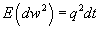 ,
,
where q2 is a model parameter. In the absence of a measurement
correction, the variance of acceleration grows linearly with time. We selected
a value for q2 of (264
ft/min2)2 /min = (3 mph/min)2 /min using the
method described in Section 3.2.
The differential equations (3.3) are written in vector form
as follows
 ,
,
where
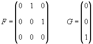 .
.
Integrating over a time interval  , we obtain the state transition model
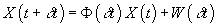 ,
,
where X(t) and  denote vehicle state
values at times t and
denote vehicle state
values at times t and  respectively.
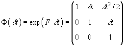
is the “transition matrix” and where
the accumulated error  has covariance
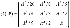 .
.
See the text following Theorem 7.1
of [10] for a discussion of integration.
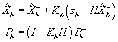
Finally, in order to run a Kalman filter/smoother we need an
initialization procedure, a method for computing an initial value for the state
vector and its associated error covariance matrix. These initial values, , are based on the initial measurement z0 (at time t0)
and measurement variance R. We set
, are based on the initial measurement z0 (at time t0)
and measurement variance R. We set 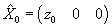 and set
 .
.
The initialization of the covariance
above is specified by a number of “hard-coded” parameters. One could attempt to
determine their “optimal” values experimentally using the techniques of Section
3.2, but we did not do so.
Now, given a sequence of measurements  at times
  , the Kalman filter transition equations are
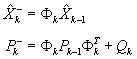 ,
,
where  is the prediction of
the state vector at the kth
step,
is the prediction of
the state vector at the kth
step, 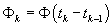 is the transition
matrix between the k-1 to the kth step, and Qk is the corresponding
transition covariance matrix. The data update equations are
is the transition
matrix between the k-1 to the kth step, and Qk is the corresponding
transition covariance matrix. The data update equations are
 ,
,
where
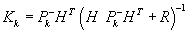 .
.
This is the set of equations for use
with real-time applications.
The equations for the smoothed estimates of state 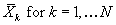 are given by
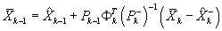 ,
,
where . See [11] for a derivation of these Kalman filter/smoother
formulas. This smoother is used for parameter estimation and post processing.
. See [11] for a derivation of these Kalman filter/smoother
formulas. This smoother is used for parameter estimation and post processing.
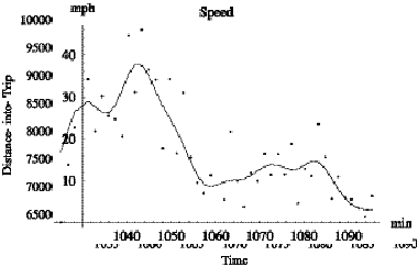
Figure 3.1 is a plot of the time series of observed and
smoothed distance-into-trip and the versus time. In Figure 3.2, the data points
are an estimate of speed based on simple differencing, and the smooth curve is
the result of the Kalman filter. Figure 3.3 is a plot of residuals, the
measurement minus the estimate, where the horizontal lines at plus and minus
500 ft correspond to the measurement variance parameter used by the filter.
Figure 3.1: Time
series of distance-into-trip.
Figure 3.2: Time
series of estimated speed.
Figure 3.3: Residuals between measurements and
estimates.
As pointed out above, our measurement and process models
depend on two parameters: the measurement variance, R, and the rate of change of the variance of process noise, q2. Using the method of
“maximum marginal likelihood,” we obtained “optimal” values for these
parameters in a number of experiments with different measurement sequences. Our
goal was not to perform an exhaustive statistical analysis, but rather just to
find some representative values that would give reasonable filter performance.
We observed that the values obtained in each experiment were roughly the same
(i.e., fluctuated around R = (500 ft)2
and q2 = (3 mph/min)2
/min).
Although the method of maximum marginal likelihood for
parameter estimation is well known to statisticians, the fact that it can be
used effectively for estimating parameters in the setting of Kalman-Bucy
filters is not widely reported. This method was first proposed in [9] where an
effective procedure is provided for evaluating the marginal likelihood
function. We briefly describe the theory.
Let Z and X denote vector-valued random variables
representing a measurement sequence and a corresponding sequence of state
vectors, and let  denote the parameter
vector (R, q2). A formula is given in [9] (Equation 4) for the
joint probability density function
denote the parameter
vector (R, q2). A formula is given in [9] (Equation 4) for the
joint probability density function  in terms of the
measurement and process models like those described above. (The symbols z and x in this context denote real-valued vectors and usage is not to be
confused with that in the preceding section.) The cited reference provides an
algorithm (Algorithm 4) which, when given a measurement vector z and parameter vector
in terms of the
measurement and process models like those described above. (The symbols z and x in this context denote real-valued vectors and usage is not to be
confused with that in the preceding section.) The cited reference provides an
algorithm (Algorithm 4) which, when given a measurement vector z and parameter vector  , simultaneously computes the maximum likelihood estimate for
the state vector sequence (the Kalman smoother estimate),
, simultaneously computes the maximum likelihood estimate for
the state vector sequence (the Kalman smoother estimate),
 ,
,
and evaluates the marginal density
function,
 .
.
As usual, the algorithm actually
works in terms of the negative logs of the various probability densities.
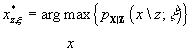
In each of our experiments, we used the cited algorithm to
define an objective function  , that depends on the measurement sequence z, and then used Powell’s conjugate
direction minimization algorithm (Chapter 10, Section 5 of [12]) to find the
optimal parameter values for each measurement sequence z,
, that depends on the measurement sequence z, and then used Powell’s conjugate
direction minimization algorithm (Chapter 10, Section 5 of [12]) to find the
optimal parameter values for each measurement sequence z,
 .
.
The results presented use a set of parameters derived as
just described.
4.
Predictor
The third component in our prescription is the Predictor.
This component provides accurate predictions of transit vehicle behavior. As
indicated in Figure 1.1, the Predictor is driven by reports from the Filter
(either data or temporal updates) and produces arrival/departure predictions  at a sequence of L scheduled time-points ahead of the
vehicle.
at a sequence of L scheduled time-points ahead of the
vehicle.
The most general form of the predictor provides a method for
predicting arrival/departure times at any point for a vehicle traveling on a
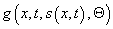
known path. To determine the travel time and the travel path x(t)
given a scheduled piecewise continuous speed function, s(x,t) where x is position
along the path and t is time, we
select a starting location and time of (x0,t0) and an ending location x1 and solve
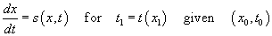 .
.
This form accounts for scheduled
travel.
However, the vehicles are affected by a variety of outside
influences. We acknowledge these effects by substituting a general functional form
 in Equation 4.1. This
form allows for dependence on the scheduled speed function s as well as such things as the statistics of observed vehicle
performance, the driver or dispatcher performance, the traffic conditions, the
changes in the measurement error, and abnormal conditions like weather and
natural disasters that depend on position and time (x,t). The travel time is
now estimated by solving
in Equation 4.1. This
form allows for dependence on the scheduled speed function s as well as such things as the statistics of observed vehicle
performance, the driver or dispatcher performance, the traffic conditions, the
changes in the measurement error, and abnormal conditions like weather and
natural disasters that depend on position and time (x,t). The travel time is
now estimated by solving
 ,
,
where the vector  represents the
parameters necessary for
represents the
parameters necessary for  . The vector
  might be coefficients
of models for delay, due to things like: traffic, historical observations, time
of day, weather, or bridge openings. For example,
might be coefficients
of models for delay, due to things like: traffic, historical observations, time
of day, weather, or bridge openings. For example,
 ,
,
where, f(x,t) is the historic snow behavior for the buses.
Accurate estimation of travel times is necessary for
accurate estimation of arrival times at future destinations. Additional
considerations are involved when estimating trip departure times or departures
after a layover. In order to clarify the notions of arrival and departure, we
make the following definitions. Let x(t) be a solution to Equation 4.2, and
let x1 = x(t1).
For any  such that
  , select tolerances
  and
and  and define the predicted arrival time at
  to be
to be
and the predicted departure time at  to be
to be
 .
.
In practice, we set  when
when  corresponds to a
“passing” time-point (i.e., a point between layovers). At a layover, however,
we require
corresponds to a
“passing” time-point (i.e., a point between layovers). At a layover, however,
we require  to ensure that a
correct estimate of departure time is computed.
to ensure that a
correct estimate of departure time is computed.
5.
Examples
To demonstrate the generalized algorithm, we present three
examples. The first example uses schedule data from Tri-Met to estimate s(x,t) and demonstrates that the popular
“schedule deviation” algorithms are degenerate forms of the generalization
presented here. The second example uses data from Seattle roadways to construct
 and shows the
complexity of the trajectory for the solution, as well as demonstrating the
need for the general form presented here. The third example uses Tri-Met AVL
and schedule data to demonstrate that the predictions provided by the
methodology suggested here are statistically far superior to the schedule
information.
and shows the
complexity of the trajectory for the solution, as well as demonstrating the
need for the general form presented here. The third example uses Tri-Met AVL
and schedule data to demonstrate that the predictions provided by the
methodology suggested here are statistically far superior to the schedule
information.
In this example, we demonstrate that the “schedule
deviation” approach to prediction is a simplified form of the general approach
presented here. To accomplish this, we define a speed function sb(x,t) based only on
schedule data such that the procedure described above computes the same
predictions as the schedule deviation procedure.
The basic idea behind the schedule deviation approach is
that it predicts arrival/departure time at time-points ahead of the vehicle
simply by adding the schedule time for the time-point to the current
interpolated schedule deviation of the vehicle. So, if the current deviation is , then this is the predicted deviation for future time-points.
This description is an over-simplification as special logic
is required to correct the predicted deviation when predicting time of
departure from a layover time-point, or a start trip time-point, or points on
beyond these. For example, the logic involved to correct deviation for a
layover departure is the following: let ta
denote the scheduled time of arrival at the layover, let td denote the scheduled time of departure, and let denote the current value for schedule deviation. If
  , then zero the deviation,
 ; otherwise, decrement the deviation,
 .
.
In order to define the speed function that corresponds to
the schedule deviation approach to prediction, we introduce the notion of distance-into-block. Recall that a
Tri-Met schedule can be represented as a series of trips making up an overall
block of work that a transit driver performs in a day. On observing the
location of a vehicle in space and time, we can translate that to a location on
a block of trips using a single parameter, distance-into-block
x, defined as follows. Suppose the point lies on the kth trip of the block and its distance-into-trip is d. Then distance-into-block for this
point is defined as the sum of the lengths of the preceding k-1 trips plus d. The trajectory for a vehicle in x-t space can be imagined
by stacking successive trips in the x-direction.
We define the scheduled trajectory of
a block to be the piece-wise linear curve in x-t space that joins
consecutive scheduled time-points.
We first define a simple piece-wise constant function,  , which we will then modify around each layover to produce
the desired function,
, which we will then modify around each layover to produce
the desired function,  . Let
. Let  be the sequence of
times and
be the sequence of
times and  be the corresponding
sequence of x-coordinates for every
scheduled time-point on the block. Then
be the corresponding
sequence of x-coordinates for every
scheduled time-point on the block. Then  for every k, and equality holds only at layover
points. Note that for every distance-into-block x there is a unique k
such that
for every k, and equality holds only at layover
points. Note that for every distance-into-block x there is a unique k
such that  . Define
  as follows:
 .
.
Now, modify this function in the
vicinity of every layover xk
= xk+1 as
follows:
 .
.
Figure 5.1 presents an example contour plot of sb(x,t) created as just
described, where darker is slower. Each of the bands of constant speed results
from the schedule based speed approximation in Equation 5.1. Further, a layover
is represented by the black or zero speed region located at 40,000 feet. The
trajectories of the solutions of Equation 4.1 are shown as white bands. The
trajectories represent the predicted location of the vehicle as a function of
space and time. Each of the three trajectories represents a vehicle with a
different starting time. The earliest or left-most travels through space and
time until it reaches the distance-into-trip where a layover is scheduled; it
then sits still until the layover has expired and continues on its way. The
middle trajectory is a vehicle that starts later than the first one and also
enters the layover. This vehicle then leaves the layover at the scheduled time
such that both the first and second solutions are the same after the layover.
The latest or right-most trajectory is a vehicle that does not arrive at the
layover location with sufficient time to stop. If the left-most trajectory
represents the planned behavior for the trip, the right-most
represents a vehicle that is late but becomes less so when it bypasses a
layover.
Figure 5.1:
Schedule based s(x, t)
and solution trajectories.
Figure 5.2: Contour plot of speed, darker is slower.
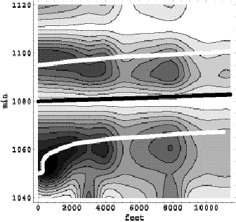
To demonstrate the importance of accurate knowledge of the
speed function to travel time estimation, we present an example of using the
algorithm with a version of the speed function  constructed using
probe vehicle data that provide speed estimates on roadways on which the
transit vehicles travel. Figure 5.2 is a contour plot of speed
constructed using
probe vehicle data that provide speed estimates on roadways on which the
transit vehicles travel. Figure 5.2 is a contour plot of speed  , a function of time and space, where the darker internal
regions are slower speeds.
, a function of time and space, where the darker internal
regions are slower speeds.
To estimate travel times given this speed function, Equation 4.2 is solved
numerically using Euler’s method. The two heavy white lines and the central
heavy black line in Figure 5.2 are the trajectories of three solutions, and the
shape of the trajectory depends heavily on the shape of the speed function. In
particular, note the character of the bottom, heavy white line that traverses a
period and region that has slow speeds. This demonstrates that to accurately
estimate travel-time, speed must be an explicit function of space and time. For
example, to estimate the travel time between two points as a function of time,
we select a start time t0
and solve Equation 4.1 for time t1
subject to constraints x(t0) = 0 feet and x(t1)
= 11,000 feet to obtain travel time t1
- t0. Figure 5.3 shows a
plot of the travel times for this stretch of road as a function of departure
time. The largest travel time peak, found at 1050 minutes, is associated with
the bottom solution trajectory in Figure 5.2.
Figure 5.3: Travel time as a function of departure time.
In our third example, we present the results of making
optimal estimates of the arrival/departure time of transit vehicles. Predicting
the future is always a challenging activity, and validating the effectiveness
of our predictions is an important measure of the success of the methodology
presented.
To compare the predictions with the vehicle behavior, we compare the prediction
to the actual arrival time. To accomplish this, we need to estimate actual
arrival time. As we are tracking the vehicle irregularly, there is no guarantee
that the location will be reported just as the vehicle arrives. To get an
estimate of the real arrival, we record the location report just before arrival
and just after arrival and linearly interpolate the actual arrival time (Ta). The implementation is
continuously predicting the arrival as a function of both space and time. We
create a deviation between the predicted and actual arrival as a function of
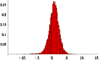
time. We then histogram and normalize the resulting deviations to create a
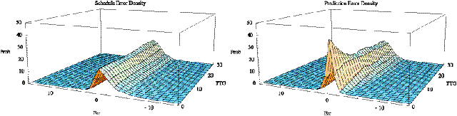
probability surface in space and time. The right side of Figure 5.4 shows the
probability of deviation of the prediction from actual, in minutes, on the
front axis (-10 to 10), and the time until arrival for which the prediction was
made on the side axis (0 to 30). A similar function for the relationship
between the schedule and the actual behavior is shown on the left side of
Figure 5.4. The surfaces in Figure 5.4 were created using the predictions made
over the course of the entire day on September 12, 2000. Comparing these two
surfaces suggests that prediction with dynamic information has 2 - 4 times
smaller errors than using the schedule alone. This demonstrates that for
transit riders using the predictive methodology presented here, there is a
significant gain in information over using just the schedule.
Figure 5.3: Probability of correct predictions mad by
the schedule on the left
and the algorithm presented on the right.
In this section, we present some results obtained by
processing Tri-Met AVL data for the week of 9/11/2000 - 9/15/2000. This data
set contained 42,618 samples for 98 trains (i.e., blocks). Each sample
consisted of the following information:
(date, route number, train, deviation, time, longitude,
latitude).
The deviation field, which is not
part of a “raw” AVL report, was computed by Tri-Met in a data post-processing
step. In most cases, it agrees closely with the negative interpolated deviation
computed by our Tracker. (Thus, a negative deviation reported by Tri-Met
indicates a late vehicle, while a positive deviation indicates an early one.)
Similarities and differences are discussed in Section 6.4 below.
Before feeding this data set into the Tracker/Predictor
pipeline, we partitioned it by day and by train and performed some elementary
analysis.
We performed some visual checks on the validity of the Oregon North state-plane
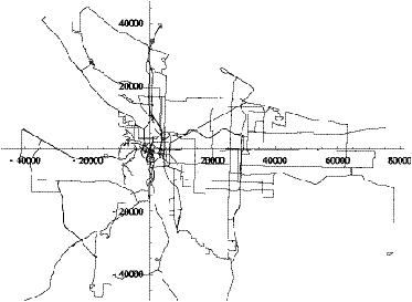
transformation we implemented using the algorithm specified in [7]. Figure 6.1
is a state-plane map showing patterns in the Tri-Met database which clearly
resembles a road map of Portland.
Figure 6.1: State-plane map of Portland bus routes.
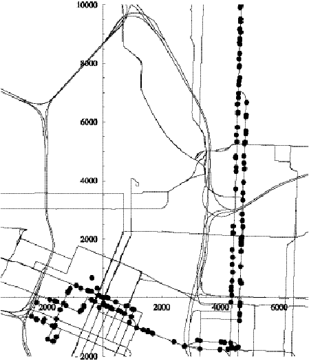
Figure 6.2 shows a superposition of transformed reports from train 668 (route
6, Martin Luther King Jr. Blvd.) on a region of this map. Visual comparison of
this image with the map for route 6 (www.tri-met.org/schedule/r006.htm) shows
that we are transforming report data correctly.
Figure 6.2: Reports from train 668.
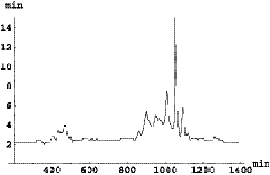
The Tracker and Kalman filter work best when the report rate
is high. For each day, we sorted the trains by number of samples and identified
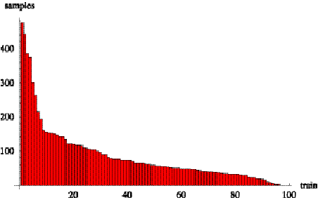
trains with large sample sets and high report rates. Figure 6.3 is a plot of
the number of samples per train, ordered from greatest to least, for day
9/11/2000.
Figure 6.3:
Distribution of the number of samples per train on day 9/11/2000.
There are 8,473 samples.
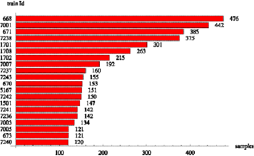
The first 20 trains provide over 50% of the samples. These trains are
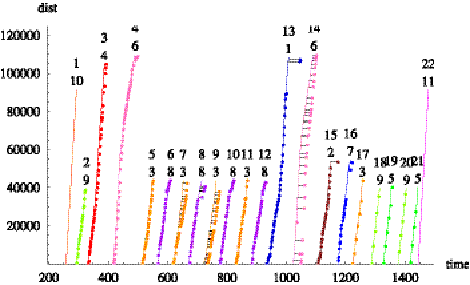
identified in Figure 6.4 below. Train 668 has the maximum number of samples,
476, while train 7240 has only 120 samples.
Figure 6.4: Trains with large sample sets on day
9/11/2000.
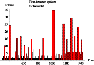
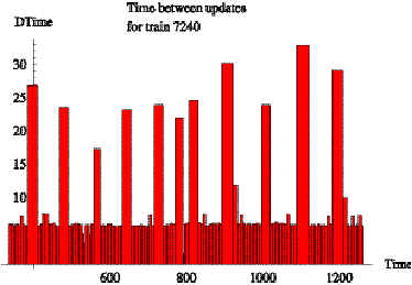
Figures 6.5 and 6.6 are bar graphs showing the time between reports (minutes)
for trains 668 and 7240 as a function of time (minutes into day). Ignoring the
large bars, we see that train 668 reports at a nominal rate of once every 2
minutes up until time 1200 minutes ( = 8 p.m.) and then continues reporting
once every 6 minutes, while train 7240 regularly reports once every 6 minutes.
Except for the bar of height 35 at time 1000 in Figure 6.5, the large bars in
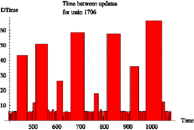
both figures correspond to layovers between trips. Figure 6.7 is a chart of
time between reports for train 1706 which has only 66 samples and is ranked 45th
in the order by sample size.
Figure 6.5: Time
between reports for train 668 on day 9/11/2000.
Figure 6.6: Time between reports for train 7240 on day
9/11/2000.
Figure 6.7: Time
between reports for train 1706 on day 9/11/2000.
In this section, we show several trip/distance-into-trip
assignments produced by the Tracker and discuss some interesting special cases.
Figures 6.8, 6.9, and 6.10 show time-series plots of distance-into-trip for
trains 668, 7240, and 1706 respectively on day 9/11/2000.
Figure 6.8: Time series of distance into trip for train
668 on day 9/11/2000.
Figure 6.9: Time
series of distance-into-trip for train 1724 on day 9/11/2000.
Figure 6.10: Time series of distance-into-trip for train
1706 on day 9/11/2000.
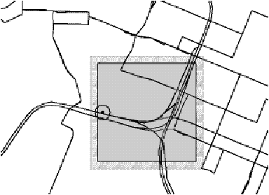
Figure 6.11 shows a close-up of a problem area on train 668
at the end of trip 13 and the start of trip 14. Note that there is a 35-minute
gap in the trip assignments starting at approximately t=1000 (i.e., 4:40 PM) This is primarily due to a gap in AVL
reports as can be observed in Figure 6.5. Our Tracker rejected several reports
and made two errant trip assignments as explained below.
Figure 6.11:
Train 668 gap in trip assignment.
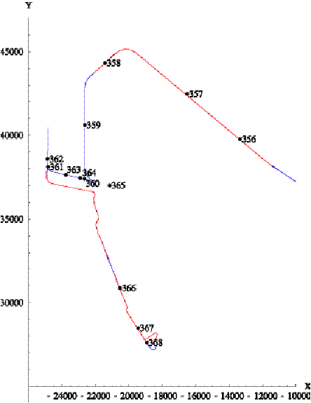
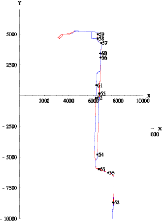
Figure 6.12 shows reports 356 through 368 and the
superposition of the patterns for trips 13 and 14. Trip 13 ends on the
turn-around loop at the bottom of the figure. Except for this loop, trip 14 is
the reverse of trip 13 in this region. Reports 356 through 362 indicate normal
progression along trip 13. However, instead of continuing forward (along
Rivergate road), reports 363 through 365 indicate that the vehicle turned
around. The Tracker rejected report 363 for this reason. Report 364 is received
after the 35-minute delay, and the Tracker finds two candidate trip assignments:
either the vehicle is 86,700 feet into trip 13 and is 40 minutes late, or it is
21,700 feet into trip 14 and 3 minutes late. Because of the disruption in
reports, the Tracker selects the latter assignment as most reasonable. Report
365 is rejected since it is too far away in distance from either trip. Report
366 is erroneously assigned to trip 14, but then the Tracker recovers and
correctly assigns reports 367 and 368 to trip 13.
Figure 6.12: Pattern for train 668.
In this section, we compare Tri-Met reported deviation with
that computed by the Tracker. For the most part they are approximately the
same, with occasional discrepancies at the start or end of trips.
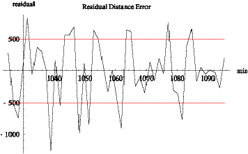
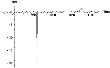
The case of train 7234 is typical. Figure 6.13 shows a spike
at time 959. This occurs on sample 37, which the Tracker assigned to trip 10
with distance 0 and deviation -3. Thus, the Tracker determined that the vehicle
was 3 minutes late to start trip 10, see Figure 6.14. The reported deviation on
this same sample was -24 indicating that the bus is 24 minutes late at the end
of trip 9. We believe the Tracker made the “correct” determination since the
vehicle appears to have arrived at
the end of trip 9 at about time 940.
Figure 6.13:
Difference of reported and computed deviation for train 7234 on day
9/11/2000.
Figure 6.14: Time series of distance-into-trip for train
7234 on day 9/11/2000.
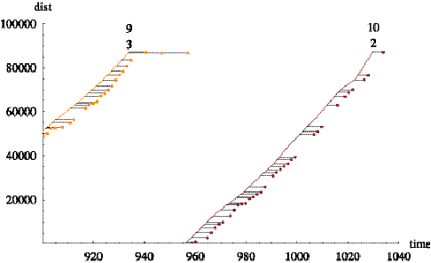
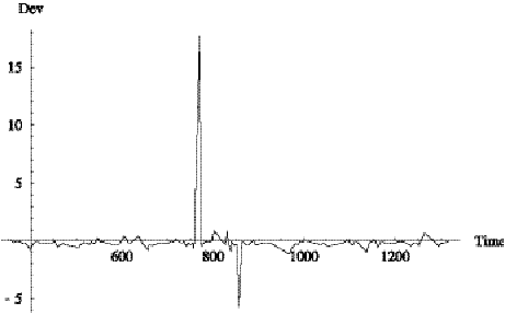
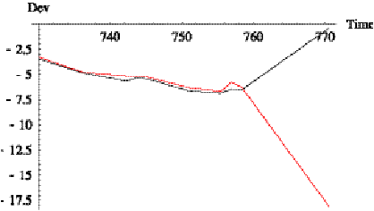
The case of train 7003 is more interesting. Figure 6.15
shows a tall spike at time 771. This occurs on sample 37, which the Tracker assigned
to trip 10 with distance 33,623 and deviation -18. Thus, the Tracker determined
that the vehicle was 18 minutes late at this point, see Figure 6.16. The
reported deviation was 0, suggesting that perhaps the vehicle is on the next
trip. However, Figure
6.17 shows the sample to lie on trip 10, and Figure 6.18 shows that it cannot
be on trip 11.
Figure 6.15:
Difference of reported and computed deviation for train 7003 on day
9/11/2000.
Figure 6.16: Comparison of reported and computed
deviation for train 7003
on trip 10 on day 9/11/2000.
Figure 6.17:
Superposition of samples of train 7003 on trips 10 and 11 on day
9/11/2000.
Figure 6.18: Sample 59 for train 7003 is not on trip 11
on day 9/11/2000.
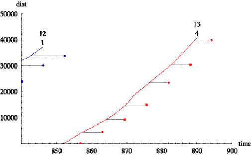
The next big spike occurs on sample 75. The reported deviation was -11, which
is consistent with vehicle arriving late at the end of trip 12. The Tracker
assigned the report to trip 13 with a deviation of -5, indicating that the
vehicle was late to depart trip 13, see Figure 6.19. Either interpretation is
probably correct.
Figure 6.19: Time series of distance-into-trip for train
7003 on trips 12 and 13 on day 9/11/2000.
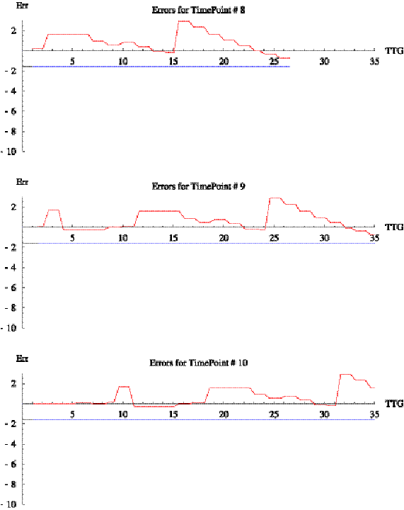
Figure 6.20 shows three examples of the absolute error in
the prediction as a function of time before arrival. This demonstrates the quality
of the prediction up to 35 minutes before arrival.
Figure 6.20: Prediction error as a function of time
before arrival.
In order to test the efficacy of the algorithmic approach in the face of
adverse conditions, we have identified a set of blocks that cross the Hawthorne
Bridge. This bridge is opened occasionally for river traffic, and the delays
caused by unscheduled opening are used to simulate adverse conditions.
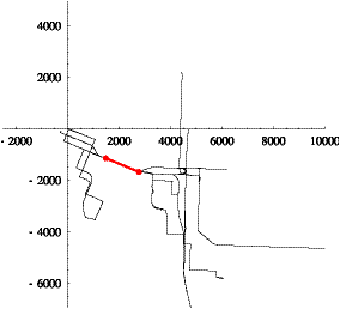
Figure 7.1: Hawthorne Bridge location on multiple blocks
of scheduled transit work.
This effort was done in coordination with Portland State
University (PSU). The researchers at PSU suggested that the routes 6, 14, 31,
32, 33, 63, 99, 104, and 110 be the focus of the analysis. We identified the geodetic
coordinates of the end points of the Hawthorne Bridge (N45.51378, W122.67300;
N45.51241, W122.66789) and mapped these to State Plane coordinates. All spatial
calculations are done in the rectangular Oregon North State Plane coordinate
system. The TPI’s containing the bridge are identified using a ‘closest point
to arc’ algorithm, as described in Appendix B and examining the TPI arcs for
the selected routes in the schedule database. There are 27 TPI’s in the
schedule data for these routes that cross the bridge. Figure 7.1 is a
two-dimensional plot of the patterns from the Tri-Met schedule that cross the
bridge. The bridge, which is approximately 1,400 feet long, is shown as the
heavier line with dots at either end, where downtown Portland is to the left of
the bridge.
Having identified the spatial TPI’s of interest, we selected
the trips that contain these TPI’s from the schedule information for November
2000 which was provided to us by Tri-Met for evaluation.
Tri-Met also provided AVL information for the fleet for
November 2000. This AVL data is composed of lists of time-tagged geodetic
locations containing time, latitude, longitude, and train number for each train
for all days in November. In order to match the AVL data to the schedule, we
used the trip assignment algorithm described in Section 2.4. After having
performed this assignment, we augmented the AVL geodetic data with Oregon North
State Plane coordinates (x,y) and schedule-relative information
corresponding to the train’s block: trip id, distance-into-trip, and schedule
deviation, where “schedule deviation” is defined as the difference of
interpolated schedule time (corresponding to distance-into-trip) and reported
AVL time. Therefore, a negative deviation indicates that a bus is behind schedule.
Bridge opening data was provided to us by PSU researchers.
The data was provided in tabular form and contained the date, opening time,
closing time, and the duration of the opening with time precision to one
minute.
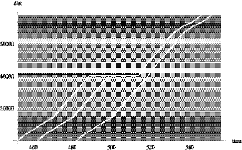
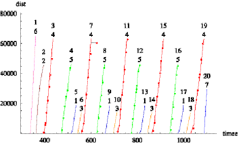
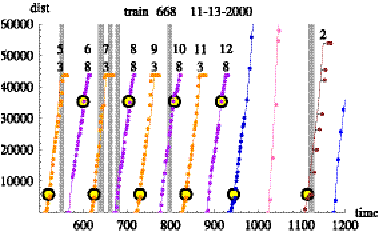
Figure 7.2 combines the AVL data, the schedule data, and the
bridge opening data for train 688 on 11/13/2000. The vertical axis is the
distance into the trip and the horizontal axis is the time of day in minutes,
where midnight is at zero minutes and 1440 minutes is 24 hours later. The lines
represent the schedule information. The numbers above each line represent the
trip number for the day (top number) and the pattern number (bottom number). So
the right leftmost trip, the fifth trip of the day, begins at approximately 500
minutes (8:20 AM) and proceeds approximately 45,000 feet on pattern three
before beginning the sixth trip of the day at 570 minutes (9:30 AM) on pattern
eight. The train repeats the spatial patterns three and eight over the next few
trips. Overlaid on the schedule information are points indicating the distance
into the trip as constructed from the AVL data. The “schedule deviation” is the
horizontal distance between the schedule line and any AVL observation where a
point to the right of the line indicates that the vehicle is late relative to
the schedule. The larger circles are placed on the schedule line at the
distance into the trip where the bus would begin crossing the bridge. Finally,
the gray vertical bars represent the time of day and duration of the bridge
openings. For the bridge opening to impact the transit service, the vehicle
must arrive at the bridge just as it is opening. This occurs only once in
Figure 7.2 on trip number fifteen during the latest or rightmost opening at
1116 minutes or 6:36 PM. In the data set analyzed, there are approximately
12,400 bridge crossings and no more than 250 were effected by bridge
openings.
Figure 7.2: Example train 688 over the course of
11/13/2000.
Vertical bars are periods when the bridge is open.
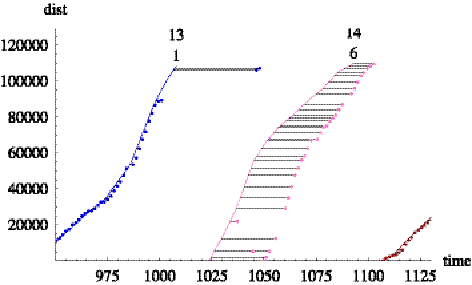
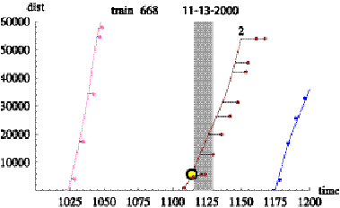
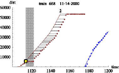
Figure 7.3 shows the impact of the bridge opening on the
fifteenth trip of train 688. The AVL data shows the bus is right on schedule
for the first point at the bottom. The bus arrives at the bridge just before it
opens and sits still for two AVL samples, causing the AVL data to move to the
right of the schedule line, and after the bridge closes, the bus continues
along the trip but with a delay.
As members of the subset of buses identified above approach
the bridge, we predict time of arrival at a nearby point on the far side of the
bridge. To do this, we use a standard schedule deviation based predictor as
described in Section 5.1. We note that the nominal AVL update rate for almost
all buses on almost all days was one sample every six to seven minutes, see
Figure 7.3. To make a prediction, an estimate of the vehicle speed is
necessary. Since the update rate is only once every 6 minutes and since, in
many cases, the bridge is close to the beginning of a trip, there were
inadequate samples to make a stable speed estimate with the Kalman filter.
Therefore, the speed estimate used in the prediction process is the one derived
from the schedule. If the update rate is on the order of one minute, as for the
data in Figure 7.4, we would have chosen to use the
filter methodology, but this rapidly updating data was largely unavailable.
Figure 7.3:
Magnified version of the fifteenth trip of train 668 that is
impacted by the bridge opening at minute 1116 (6:36 PM).
Figure 7.4: Fast update rate data suitable for use with
a Kalman filter predictor.
The prediction method used for this data set takes AVL data
for a trip with a scheduled bridge crossing and finds the last AVL sample that
is no closer than 500 feet from the start of the bridge and predicts the
arrival time corresponding to the first AVL sample that is greater than 500
feet downstream of the bridge. Figure 7.5 is a plot of the probability density
of the error made in predicting arrival downstream using the standard predictor
for all crossings. There were 12,482 samples, a mean error of 0.5 minutes, and
a standard deviation of 1.95 minutes. The trips impacted by the bridge opening
make up only two percent of all trips and thus do not bias the overall
prediction significantly.
Figure 7.5: Probability of correctly predicting the
vehicle arrival downstream
of the bridge for all bridge crossings identified.
In order to gauge the effect of bridge openings, we restricted the sample set
to bridge crossings where the predicted arrival time at the bridge was during
the bridge open time interval. Figure 7.6 shows the statistical probability
density of error using the standard predictor on this restricted set. There
were 231 samples, a mean error of -3.6 minutes, and a standard deviation of 3.4
minutes. We observe the mean error bias expected in this subset.
Figure 7.6: Probability density for correct prediction
for trips
impacted by a bridge opening.
To attempt to quantify the benefit of having real-time bridge opening
information, we modified the predictor to use the bridge opening time and the
mean duration of bridge opening to make predictions. When a bridge opening is
reported, predict the arrival time at the bridge. If this time is less than the
estimated lift closing time, open time plus nine minutes, then predict arrival
on the other side of the bridge using the deviation induced by closing time.
Figure 7.7 shows the statistical probability density of error using the
modified predictor on the restricted data set. There were 231 samples, a mean
error of 0.5 minutes, and a standard deviation of 3.5 minutes. Observe that
there are a number of ‘outliers’ in the prediction error using the modified
predictor. These are due to a number of factors, including error in recorded
bridge lift open/close times and error in prediction of arrival time at start
of bridge.
Figure 7.7: Prediction made assuming real-time bridge
opening data is available.
In this report, we present a complete paradigm for transit
arrival/departure prediction. The overall algorithm is broken into three
components, the Tracker, the Filter and the Predictor, through which the data
flows. The algorithms within each component are documented in this report, and
this provides an open reference that could be used for evaluation of a closed
or proprietary system.
The report presents results of applying the algorithms to a
small Tri-Met data set from September 2000. This example demonstrates that
there is a significant gain in information, over the schedule, that can be
provided to passengers using the AVL data with these algorithms. The computed
schedule deviation estimate by the algorithm presented appears to be superior
to the deviation provided by Tri-Met in the data set. This report also provided
a set of innovative methods for data visualization to enable the analysis and
evaluation of AVL data as well as trip assignment and schedule deviation.
Finally, we report the performance of predictions when
adverse conditions effect the bus progress. Data for buses that cross the
Hawthorne Bridge, which open occasionally, are used with the prediction scheme,
and the effect of occasional delays is quantified. The value of providing
real-time bridge opening data to the prediction algorithm is also quantified.
Real-time bridge opening information will improve the real-time predictions;
however, increasing the sampling frequency, to perhaps once per minute, for the
AVL data will have significantly more effect at improving the predictions.
1. Cathey,
F.W. and D.J. Dailey, “A Prescription for Transit Arrival/Departure Prediction
Using Automatic Vehicle Location Data,” Transportation
Research C, to appear 2002.
2. Dailey,
S.J., S.D. Maclean, F.W. Cathey, and Z. Wall, “Transit Arrival Prediction: An
Algorithm and a Large Scale Implementation,” Transportation Research Record, to appear 2002.
3. Dailey,
D.J., Z. Wall, S.D. Maclean, and F.W. Cathey, “An algorithm and Implementation
to Predict the Arrival of Transit Vehicles,” Proceedings of the IEEE Intelligent Transportation Systems Conference,
October 2000.
4. Wall,
Z. and D.J. Dailey, “An Algorithm for Predicting Arrival Time of Mass Transit
Vehicles Using AVL,” Proceedings of the
Transportation Research Board Annual Meeting, January 1999.
5. Dailey,
D.J., D. Meyers, and N. Fiedland, “A Self Describing Data Transfer Methodology
for ITS Applications,” Transportation
Research Record No. 1660, pp.
140-147, 1999.
6. Joint
AASHTO/ITE/NEMA Standards Publication, Transit Communications Interface Profiles
(TCIP) Framework Document (NTCIP 1400), Draft 97.01.02, Institute of
Transportation Engineers, 1999.
7. Stern,
J.E., State Plane Coordinate System of
1983, NOAA Manual NOS NGS 5, January 1989.
8. Charniak
and McDermott, Introduction to Artificial
Intelligence, Addison-Wesley, 1984.
9. Bell,
B.M., “The Marginal Likelihood for Parameters in a Discrete Gauss-Markov
Process,” IEEE Transactions on Signal
Processing, vol. 48, no. 3, March 2000.
10. Jazwinski, A.H.,
Stochastic Processes and Filtering Theory, Academic Press, 1970.
11. Tun, F., H.E.
Rauch, and C.T. Striebel, “Maximum Likelihood Estimates of Linear Dynamic
Systems,” American Institute of
Aeronautics and Astronautics Journal, vol. 3, pp. 1445-1450, August 1965.
12. Anderson, B.D.O.
and J.B. Moore, Optimal Filtering,
Prentice-Hall, Inc., 1979.
Appendix A:
Searching a Geographic Data Set Using Tiles
In order to create an efficient procedure for indexing and
sorting a large geographic data set, we introduce a new a two-dimensional
indexing structure that permits rapid calculation of subsets of geo-points.
This structure consists of a regular grid of non-overlapping rectangular
regions (tiles) superimposed over the entire region of operation of the transit
fleet. Each tile is uniquely determined by two indices, and given the grid
origin and tile dimensions, the indices of the tile containing any reported
vehicle location can be computed quickly using simple arithmetic with no
searching involved. We relate the tiles to TPI’s as follows. For each tile T form an associated “inflated” tile  by adding a “halo” of
width equal to the maximum expected position measurement error R. For every TPI in the database,
associate to it the set of tiles {Ti}
such that the TPI intersects the corresponding inflated tile
by adding a “halo” of
width equal to the maximum expected position measurement error R. For every TPI in the database,
associate to it the set of tiles {Ti}
such that the TPI intersects the corresponding inflated tile  , and also associate the corresponding intersection sub-paths
of the TPI with
, and also associate the corresponding intersection sub-paths
of the TPI with  . It follows that a circular neighborhood N(p,
R) of an arbitrary point p on a tile T can possibly intersect a given TPI only if that TPI is associated
with tile T.
. It follows that a circular neighborhood N(p,
R) of an arbitrary point p on a tile T can possibly intersect a given TPI only if that TPI is associated
with tile T.
Figure A.1 illustrates the notions of circular neighborhood, tile, and
associated inflated tile. The neighborhood has a radius of 150 feet, and the
tile has width and height of 2,000 feet.
Figure A.1: A point on a tile.
We describe a simple algorithm for computing distance r from a point p to a
line segment  and for computing
distance d into the segment for point
q, which corresponds to this distance.
The idea is to use properties of the vector dot-product and consider the
projection of p onto the directed
line running through q1
and q2, see Figure B.1.
and for computing
distance d into the segment for point
q, which corresponds to this distance.
The idea is to use properties of the vector dot-product and consider the
projection of p onto the directed
line running through q1
and q2, see Figure B.1.
Figure B.1: Distance from point to line segment.
Let v = q2 - q1 and w = p - q1
and recall the dot-product formula  where
where  is the length of w,
  is the length of v, and
  is the angle between w and v. The projection of w
onto the line determined by v is
given
is the angle between w and v. The projection of w
onto the line determined by v is
given  . There are 3 cases to consider.
1. If  0, then
  is obtuse and the
projection of p lies before q1, and hence, q1 is the closest point to p. Thus,
is obtuse and the
projection of p lies before q1, and hence, q1 is the closest point to p. Thus,  and d = 0.
2. If  , then p projects
onto the segment. Hence,
, then p projects
onto the segment. Hence,  and
and  .
.
3. If  , then the projection of p
lies beyond q2, and hence,
q2 is the closest point on
the segment to p. Hence,
, then the projection of p
lies beyond q2, and hence,
q2 is the closest point on
the segment to p. Hence,  and
and  .
.
(Note that when this algorithm is applied to a chain of
segments in the search for a closest point, step 3 can be skipped as redundant
on all segments, except possibly the last one.)