MBTC 1099
MODELING TRAFFIC FLOWS AND CONFLICTS AT ROUNDABOUTS
PREPARED BY:
Dr. Eugene R. Russell, P.E., Civil Engineering, Kansas State University
Dr. Margaret Rys, Industrial Management and Safety Engineering, Kansas State University
Greg Luttrell, P.E., Graduate Research Assistant, Kansas State University
FUNDED BY:
Mack-Blackwell Rural Transportation Center, University of Arkansas
Kansas State University
City of Manhattan, Kansas
February 2000
TABLE OF CONTENTS
Table of Contents *
Table of Figures *
Table of Tables *
CHAPTER 1 – Executive Summary *
Section 1.1 - Introduction *
CHAPTER 2 - The Manhattan Roundabout *
Section 2.1 – Roundabout Geometry *
Section 2.2 – Hourly Traffic Volumes *
Section 2.3 – Mini Traffic Circles in Manhattan, Kansas *
Section 2.4 - Local Print Media Coverage *
Section 2.4.1 - Focus of Local Print Media *
Section 2.4.2 – Article Summaries – Roundabouts *
CHAPTER 3 – Experimental Design *
Section 3.1 – Video Data Collection *
Section 3.2 – Manual Data Collection *
Section 3.3 – Comparable Intersections *
Section 3.4 – Data Analysis *
CHAPTER 4 – Comparable Intersections *
Section 4.1 – Dickens Avenue/ Wreath Avenue (DW) *
Section 4.2 – Juliette Avenue/ Pierre Street (JP) *
Section 4.3 – Comparison of Traffic Volumes at the Three Study Intersections *
CHAPTER 5 – Safety *
Section 5.1 – Literature Review *
Section 5.1.1 - Safety of Roundabouts *
Section 5.1.2 - Bicycle and Pedestrian Safety *
Section 5.1.3 - Bicycle and Pedestrian Design *
Section 5.2 – Crash Review *
Section 5.4 – Conflict Analysis – Literature Review *
Section 5.5 – Conflict Analysis – CG, DW and JP *
Section 5.5 – Intersection Travel Speed *
Section 5.6 – Summary of Safety Evaluation *
CHAPTER 6 – Traffic Volume and Delay *
Section 6.1 – Daily Traffic Volumes *
Section 6.2 – Intersection Delay *
Section 6.3 - Delay at the Manhattan Roundabout *
CHAPTER 7 – SIDRA Analysis *
CHAPTER 8 – Statistical Analysis of Roundabout and Comparable Intersections – Analysis I *
Section 8.1 – Statistical Analysis of SIDRA Hourly Traffic Values (I) *
Section 8.2 – Statistical Analysis of SIDRA Output for Roundabout and Comparable Intersections (I) *
Section 8.2.1 – Statistical Analysis of 95 Percentile Queue (I) *
Section 8.2.2 – Statistical Analysis of Average Delay (I) *
Section 8.2.3 – Statistical Analysis of Maximum Approach Delay (I) *
Section 8.2.4 – Statistical Analysis of Proportion Stopped (I) *
Section 8.2.5 – Statistical Analysis of Maximum Proportion Stopped (I) *
Section 8.2.6 – Statistical Analysis of Degree of Saturation (I) *
Section 8.2.7 – Summary of Statistical Analysis of SIDRA Output (I) *
CHAPTER 9 – Statistical Analysis of Candlewood Drive/Gary Avenue Intersection – Analysis II *
Section 9.1 – 95 Percentile Queue at Candlewood Drive/Gary Avenue (II) *
Section 9.2 – Average Delay for Candlewood Drive/Gary Avenue (II) *
Section 9.3 – Maximum Approach Delay for Candlewood Drive/Gary Avenue (II) *
Section 9.4 – Proportion Stopped for Candlewood Drive/Gary Avenue (II) *
Section 9.5 – Maximum Proportion Stopped for Candlewood Drive/Gary Avenue (II) *
Section 9.6 – Statistical Analysis of Degree of Saturation (II) *
Section 9.7 – Summary of Statistical Analysis II *
CHAPTER 10 – Summary and Conclusions *
Section 10.1 – Study Summary *
Section 10.2 – Conclusions *
TABLE OF FIGURES
Figure 1 - Roundabout in Manhattan, Kansas *
Figure 2 - United States Roundabouts and Entering Traffic Volumes *
Figure 3 - Candlewood Drive/Gary Avenue - Approach Traffic Counts *
Figure 4 - Cumulative Frequency Distribution of Traffic Counts - Candlewood Drive/Gary Avenue *
Figure 5 - Manhattan, Kansas Mini Traffic Circle *
Figure 6 - Omnidirectional Video Camera Mounted to Street Light Pole *
Figure 7 - Video Recording Assembly *
Figure 8 - Dickens Avenue/Wreath Avenue – Total Approach Traffic Counts *
Figure 9 - Cumulative Frequency Distribution of Traffic Counts - DW *
Figure 10 - Juliette Avenue/Pierre Street – Total Approach Traffic Counts *
Figure 11 - Cumulative Frequency Distribution - Juliette Avenue/Pierre Street *
Figure 12 - Comparison of Entering Volumes at the Three Study Intersections *
Figure 13 – Standard Intersection Conflict Points *
Figure 14 - Roundabout Intersection Conflict Points *
Figure 15 – 95 Percentile Queue Values (I) *
Figure 16 - Average Vehicle Delay (I) *
Figure 17 - Maximum Approach Average Vehicle Delay (I) *
Figure 18 - Proportion Stopped (I) *
Figure 19 - Maximum Approach Proportion Stopped (I) *
Figure 20 - Degree of Saturation (I) *
Figure 21 – 95 Percentile Queues (II) *
Figure 22 - Average Vehicle Delay (II) *
Figure 23 - Maximum Approach Average Vehicle Delay (II) *
Figure 24 - Proportion Stopped (II) *
Figure 25 - Maximum Approach Proportion Stopped (II) *
Figure 26 - Degree of Saturation (II) *
TABLE OF TABLES
Table 1 - Roundabout Design Speed and Application *
Table 2 - Count Data - Candlewood Drive/Gary Avenue *
Table 3 - Candlewood Drive/Gary Avenue Approach Counts *
Table 4 - Candlewood Drive/Gary Avenue 85 Percentile Approach Speeds *
Table 5 - Comparable Intersection Selection Criteria *
Table 6 - Intersection Measures of Effectiveness *
Table 7 - Dickens Avenue/Wreath Avenue Approach Traffic Counts *
Table 8 - Dickens Avenue/Wreath Avenue 85 Percentile approach Speeds *
Table 9 - Dickens Avenue/Wreath Avenue Traffic Count Data *
Table 10 - Juliette Avenue/Pierre Street approach Traffic Counts *
Table 11 - Juliette Avenue/Pierre Street 85 Percentile approach Speeds *
Table 12 - Juliette Avenue/Pierre Streeet Traffic Count Data *
Table 13 - Safety and Operational Concerns of Roundabouts *
Table 14 - Crash Records Before and After Roundabout Installation *
Table 15 - Before and After Crash Costs at Roundabout *
Table 16 - Basic Intersection Conflicts - Standard Intersection and Roundabout Control *
Table 17 - Statistical Test Summary Overview *
Table 18 - Statistical Test Summary of SIDRA Traffic Volumes (I) *
Table 19 - Summary Statistics of SIDRA Traffic Volumes (I) *
Table 20 - 95 Percentile Queue Values (I) *
Table 21 - Statistical Test Summary of 95 Percentile Queue (I) *
Table 22 - 95 Percentile Mean and Standard Deviation (I) *
Table 23 - Average Vehicle Delay (I) *
Table 24 - Statistical Test Summary for Average Vehilcle Delay (I) *
Table 25 - Average Vehicle Delay Mean and Standard Deviation (I) *
Table 26 - Maximum Approach Avenage Vehicle Delay (I) *
Table 27 - Statistical Test Summary for Maximum Approach Delay (I) *
Table 28 - Maximum Approach Delay Mean and Standard Deviation (I) *
Table 29 - Proportion Stopped (I) *
Table 30 - Statistical Test Summary for Proportin Stopped (I) *
Table 31 - Proportion Stopped Mean and Standard Deviation (I) *
Table 32 - Maximum Approach Proportion Stopped (I) * Table 33 - Statistical Test Summary for Maximum Approach Stopped (I) *
Table 34 - Maximum Proportion Stopped Mean and Standard Deviation (I) *
Table 35 - Degree of Saturation (I) *
Table 36 - Statistical Test Summary for Degree of Saturation (I) *
Table 37 - Degree of Saturation Mean and Standard Deviation (I) *
Table 38 - Summary of MOE Statistical Results - Analysis I *
Table 39 - 95 Percentile Queues (II) *
Table 40 - Statistical Test Summary for 95 Percentile Queues (II) *
Table 41 - 95 Percentile Queue Mean and Standard Deviation (II) *
Table 42 - Average Vehicle Delay (II) *
Table 43 - Statistical Test Summary for Average Delay (II) *
Table 44 - Average Delay Mean and Standard Deviation (II) *
Table 45 - Maximum Approach Average Vehicle Delay (II) *
Table 46 - Statistical Test Summary for Maximum approach Delay (II) *
Table 47 - Maximum Approach Delay Mean and Standard Deviation (II) *
Table 48 - Proportion Stopped (II) *
Table 49 – Statistical Test Summary for Proportion Stopped (II) *
Table 50 - Proportion Stopped Mean and Standard Deviation (II) *
Table 51 - Maximum Approach Proportion Stopped (II) *
Table 52 - Statistical Test Summary for Maximum Approach Stopped (II) *
Table 53 - Maximum approach Stopped Mean and Standard Deviation (II) *br> Table 54 - Degree of Saturation (II) *
Table 55 - Statistical Test Summary for Degree of Saturation (II) *
Table 56 - Degree of Saturation Mean and Standard Deviation (II) *
Table 57 - Summary of MOE Statistical Results - Analysis II *
Table 58 - Summary of MOE Statistical Results - Analysis I *
Table 59 - Summary of MOE Statistical Results - Analysis II *
APPENDICES
Appendix 1: Advisory Committee
Appendix 2: Annotated Bibliography
Appendix 3: Sample SIDRA Results, Candlewood Drive/Gary Avenue
Appendix 4: Sample SIDRA Results, Dickens Avenue/Wreath Avenue
Appendix 5: Sample SIDRA Results, Juliette Avenue/Pierre Avenue
Appendix 6: News Items, Manhattan (KS) Mercury
Modern roundabouts are becoming a viable intersection alternative in many United States locations. The acceptable operation of the modern roundabout depends on the location having adequate geometric characteristics (i.e.: deflection, splitter islands) and operating under the yield to the traffic in the circle priority rule. Jurisdictions within the State of Kansas are considering roundabouts in over nine locations. To provide a basis for the understanding of the operation of a modern roundabout in Kansas, a study was performed on the only existing modern roundabout in the State.
This project examined the operation of a roundabout under two comparative scenarios. The roundabout was located in Manhattan, Kansas and was constructed in the fall of 1997. Operation of the roundabout was observed from videotape recorded using a 360o video camera linked to video recording equipment. Traffic data was obtained through viewing the videotapes. Traffic count data was used as input into a computer simulation program called SIDRA (Signalized and Unsignalized Design and Research Aide). Of the evaluative outputs available, six were chosen relating to the operation of the intersection (95% queue length, average delay, maximum approach delay, proportion stopped, maximum proportion stopped, and degree of saturation). The values obtained for each of these measures of effectiveness (MOEs) were statistically tested to determine under what configuration the intersections operated better.
In the first comparison, the operation of the roundabout was measured against two comparable two-way STOP controlled intersections. The values for each of the six MOEs were obtained for the three intersections. The roundabout was found to operate statistically better than the two-way STOP intersections with respect to maximum approach delay, maximum approach stopped and degree of saturation. The roundabout was found to operate statistically worse than the two-way STOP intersections with respect to average delay. Operational conclusions were not able to be made with regard to the MOEs of 95% queue and proportion stopped.
In the second evaluation the operation of the roundabout was evaluated against the pre-roundabout two-way STOP intersection configuration, and two four-way STOP control intersection scenarios. When evaluated for average delay, the roundabout and two-way STOP performed statistically equal to each other, and better than either four-way STOP alternative. Under the remaining five MOEs (95% queue, maximum approach stopped, proportion stopped, maximum proportion stopped, and degree of saturation) the roundabout performed statistically better than the 2 and four-way STOP intersection scenarios.
Traffic conflicts were studied as a predictor of the safety of the three intersections. However, through viewing of over 180 hours of videotapes, only one traffic conflict was observed. Therefore, evaluation of the intersections was not made with regard to traffic conflicts.
Traffic crash records were obtained for thirty-six months before and twenty-nine months after roundabout installation. These crash records were examined to evaluate the change of safety of the intersection when changed to roundabout configuration. Prior to roundabout installation, the intersection experienced an average of 3 crashes per year. Of these crashes, there was an average of 1.33 injury crashes per year. In the twenty-nine months since roundabout installation, there have been no reported traffic crashes.
The Manhattan roundabout installation was found to be a good intersection control/ configuration choice.
This research project has helped to establish that even at relatively low traffic volumes; roundabout control of an intersection is beneficial. However, caution must be used in taking these results generated from examination of one roundabout site and applying them to all such sites. Much additional study is needed before the engineering community fully understands the operation and safety benefits of roundabouts compared to other intersection control types. This study should be considered a full examination of the Manhattan roundabout, and a first step toward this fuller understanding of roundabout operation.
SECTION 1.1 - Introduction
Modern roundabouts have a number of operational and physical characteristics that make them unique, and functional as a traffic control device/ intersection configuration. Old style roundabouts have been called traffic circles, rotaries and gyratories. Modern roundabouts have three primary differences from the old style roundabout: yield at entry, deflection and flare (1).
Modern roundabouts operate on the ‘yield to circulating traffic’ rule. The old method of operation was for drivers in the roundabout to yield to vehicles on the right. This resulted in traffic locking up the roundabout when volumes were heavy. By operating under the ‘yield to circulating traffic’ rule, vehicles only enter the circulating stream when there is a suitable gap. This allows the modern roundabout to continue to flow even at relatively high traffic volumes.
Modern roundabouts also have properly designed deflection of the entering traffic. The old designs treated roundabouts as weaving sections and were built to facilitate high vehicle entry and circulating speeds. Deflection slows approaching vehicles down to a speed where the safety of the roundabout is greatly enhanced. Operation speeds of modern roundabouts should be kept below 40 kilometers per hour (25 miles per hour) (2).
TABLE 1 - Roundabout Design Speed and Application
| Design Speed (kph) |
Design Speed (mph) |
Application |
| 19 – 24 |
12 – 15 |
Local and collector street intersections |
| 24 – 29 |
15 – 18 |
Collector to major arterial roads |
| 29 – 37 |
18 – 23 |
Minor to major arterial roads |
| 37 - 40 |
23 – 25 |
High speed (80 – 88 kph, 50 – 55 mph) roads including high speed rural intersections |
Source: (2)
Finally, modern roundabouts can have flared approaches. The widening of the approach road to allow for additional entrance lanes increases the flexibility of the operation for drivers and enhances the capacity of modern roundabouts.
Theoretically the operation of a roundabout is similar to a series of linked ‘T’ intersections. As such, an approaching driver can check for pedestrian/ bicycle traffic as they approach the intersection, then they have to deal with conflicting traffic from only one direction: the left. Once in the roundabout, the driver continues around until making a right turn to exit the intersection.
"Adequate deflection through roundabouts is the most important factor influencing their safe operation" (3). The deflection through the roundabout is created by both the diameter of the center island, and entrance angle created by the splitter island. The central island should be circular; however, other round shapes (i.e.: ovals) are acceptable. In general, roundabout center islands should have a diameter of 5 to 30 meters (15 – 160 feet) (3).
Splitter islands are generally raised median islands that serve many functions. While some older roundabouts were constructed with painted splitter islands, non-raised splitter islands negates many of their advantages. Splitter islands guide vehicles into the circulating roadway of the roundabout, initiating the vehicle’s deflection from the approach roadway. As such, they should be designed in conjunction with the vehicles’ curved path so that traversing vehicles have a smooth path through the roundabout. The deflection curve establishes the horizontal path of a vehicle going through the roundabout and defines the design speed of the roundabout. Therefore, the tighter the deflection curve, the slower the design speed of the roundabout (2).
Splitter islands also serve to prevent wrong way movements. They create physical barriers whereby a vehicle wishing to traverse the roundabout the wrong way would have to travel over or through the splitter island.
The approach ends of splitter islands can provide a physical narrowing of the approach roadway prior to the flare area. This narrowing of the approach road tends to slow vehicle approach speeds and alerts drivers to the upcoming roundabout. Splitter islands have a tendency to change driver expectancy as they approach the roundabout.
Finally,
"On arterial road roundabouts, the splitter island should be of sufficient size to shelter a pedestrian (at least 2.4 meters wide) and be a reasonable target to be seen by approaching traffic. A minimum total area of 8 to 10 m2 should be provided on arterial road approaches" (3).
Therefore, the splitter islands also act as pedestrian refuge islands. This allows a pedestrian to cross one direction of traffic, reach the splitter island, then cross the other. Separation of the crossing movement enhances pedestrian safety at roundabouts. The use of splitter islands for pedestrian refuge requires that they be designed to meet all applicable (including the Americans with Disabilities Act) requirements relating to pedestrian activity.
Modern roundabouts often have beautified center islands. Both the Oregon (4) and Maryland (1) State guides for roundabouts provide directions on how to safely landscape the center island so as not to compromise visibility. The landscaping of the center island allows the roundabout to function as an urban design element.
When trucks need to be accommodated at a roundabout, the design usually includes a truck apron. This is a part of the center island that is not fully raised above the circulating roadway pavement. Rather it is raised 5 to 10 cm (2 – 4 in). Truck aprons are most often constructed of a contrasting material to help differentiate them from the circulating roadway. The purpose of a truck apron is to provide an area where the rear wheels of a large vehicle can be accommodated while keeping the central island small (and therefore maintaining the needed travel path deflection).
The Australian guide to traffic engineering practice for roundabouts (3) lists a number of methods of intersection control as well as where roundabouts are appropriate and inappropriate.
"Roundabouts may be appropriate in the following situations:
- At intersections where traffic volumes on the intersecting roads are such that:
- ‘Stop" or ‘Give Way’ signs or the ‘T’ junction rule result in unacceptable delays for the minor road traffic. In these situations, roundabouts would decrease delays to minor road traffic, but increase delays to the major road traffic.
- Traffic signals would result in greater delays than a roundabout. It should be noted that in many situations roundabouts provide a similar capacity to signals, but may operate with lower delays and better safety, particularly in off-peak periods.
- At intersections where there are high proportions of right (left)-turning traffic….
- At intersections with more than four legs….
- At cross intersections of local and/or collector roads where a disproportionately high number of accidents occur involving either crossing traffic or turning movements….
- At rural cross intersections (including those in high speed areas) at which there is an accident problem involving cross traffic….
- At intersections of arterial roads in outer urban areas where traffic speeds are high and right (left) turning traffic flows are high….
- At ‘T’ or cross intersections where the major traffic route turns through a right angle….
- Where major roads intersect at ‘Y’ or ‘T’ junctions….
- At locations where traffic growth is expected to be high and where future traffic patterns are uncertain or changeable.
- At intersections of local roads where it is desirable not to give priority to either road" (3).
Parenthetical notation added by author to apply to driving on right circumstances.
The manual then proceeds to list a number of locations where roundabouts may not be an appropriate traffic control.
"
Roundabouts may be inappropriate in the following situations:
- Where a satisfactory geometric design cannot be provided due to insufficient space or unfavorable topography or unacceptably high cost of construction….
- Where traffic flows are unbalanced with high volumes on one or more approaches….
- Where a major road intersects a minor road and a roundabout would result in unacceptable delay to the major road….
- Where there is considerable pedestrian activity and due to high traffic volumes it would be difficult for pedestrians to cross the road….
- At an isolated intersection in a network of linked traffic signals….
- Where peak period reversible lanes may be required.
- Where large combination vehicles or over-dimensional vehicles frequently use the intersection and insufficient space is available to provide for the required geometric layout.
- Where traffic flows leaving the roundabout would be interrupted by a downstream traffic control which could result in queuing back into the roundabout." (3).
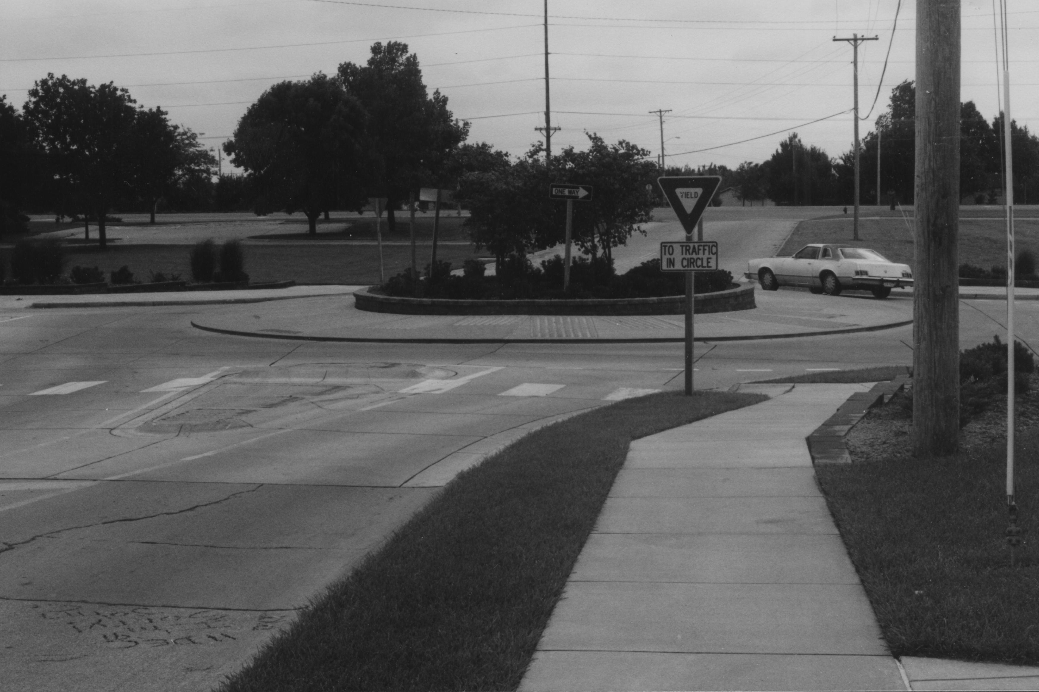
The roundabout built in Manhattan was the first modern roundabout to be built in the state of Kansas (see Figure 1). The roundabout is located at the intersection of two collector roads: Candlewood Drive/ Gary Avenue. The roundabout is adjacent to a residential area. The roundabout was completed in the fall of 1997.
FIGURE 1 - Roundabout in Manhattan, Kansas
SECTION 2.1 – Roundabout Geometry
The Manhattan roundabout controls a four-leg intersection. All approach legs are two lane roadways (one entering and one exiting) and parking is allowed on both sides of all approach roads (see Figure 1). There is one circulating lane. All approaches are controlled with a YIELD sign. Each approach has a raised splitter island and all approaches have marked crosswalks. The central island is approximately 9.1 meters (30 feet) in diameter with a 3.7 meter (12 feet) wide truck apron. The approach lane widths are generally 4.6 meters (15 feet) wide.
The roundabout is controlled by ‘yield to circulating traffic’ rule and has deflection creating a low speed curve around the central island, thereby fitting the definition of a roundabout of modern design.
SECTION 2.2 – Hourly Traffic Volumes
The Manhattan roundabout carried traffic at what can be considered to be the bottom end of the range for existing roundabouts in the United States. A National Cooperative Highway Research Program report (1998) (5) presented the hourly traffic levels at existing roundabouts from across the United States (see Figure 2). The hourly approach volumes ranged from a low of 300 vph in Las Vegas, Nevada to a high of 4,700 vph in Long Beach, California.
FIGURE 2 - United States Roundabouts and Entering Traffic Volumes
Source (5), modified to also show the Manhattan roundabout
* peak hour traffic not defined in source
The daily traffic volumes at the Manhattan roundabout ranged from 738 to 1,680 vpd on each of the four approaches. The average hourly entering volume ranged from 224 to 402 vehicles with an average of 310 vehicles (see Table 2).
TABLE 2 - Count Data - Candlewood Drive/ Gary Avenue
|
Date:
|
Day of Week:
|
Count:
|
Peak Hour Factor:
|
Max Peak Hour:
|
| 2/26/99 |
Friday |
224 |
0.78 |
287 |
| 2/27/99 |
Saturday |
230 |
0.80 |
288 |
| 1/19/99 |
Tuesday |
272 |
0.52 |
523 |
| 1/22/99 |
Friday |
277 |
0.83 |
334 |
| 2/27/99 |
Saturday |
280 |
0.79 |
354 |
| 2/18/99 |
Thursday |
285 |
0.63 |
452 |
| 1/20/99 |
Wednesday |
289 |
0.83 |
348 |
| 2/19/99 |
Friday |
293 |
0.85 |
345 |
| 1/20/99 |
Wednesday |
296 |
0.74 |
400 |
| 2/27/99 |
Saturday |
311 |
0.93 |
334 |
| 2/27/99 |
Saturday |
315 |
0.83 |
380 |
| 1/22/99 |
Friday |
320 |
0.79 |
405 |
| 1/19/99 |
Tuesday |
321 |
0.89 |
361 |
| 1/19/99 |
Tuesday |
324 |
0.86 |
377 |
| 2/27/99 |
Saturday |
330 |
0.93 |
355 |
| 2/18/99 |
Thursday |
333 |
0.67 |
497 |
| 2/27/99 |
Saturday |
344 |
0.96 |
358 |
| 2/27/99 |
Saturday |
348 |
0.77 |
452 |
| 1/21/99 |
Friday |
354 |
0.66 |
536 |
| 2/17/99 |
Wednesday |
364 |
0.82 |
444 |
| 1/19/99 |
Tuesday |
364 |
0.94 |
387 |
| 2/27/99 |
Saturday |
402 |
0.97 |
414 |
| |
|
310
|
0.80
|
387
|
|
Summary:
|
| |
Max: |
402 |
Range: |
178 |
| |
Min: |
224 |
|
|
Typical daily distribution at the roundabout intersection is shown in Table 3. These traffic counts were collected on Thursday, January 28, 1999. These hourly traffic counts are shown graphed in Figure 3.
TABLE 3 - Candlewood Drive/ Gary Avenue Approach Counts
Figure 3 - Candlewood Drive/ Gary Avenue - Approach Traffic Counts
Vehicle approach speed data was collected at the roundabout intersection. The 85 percentile speeds for approaching vehicles ranged from 43 to 48 kph (27 to 30 mph). The variation of these speeds by approach is shown in Table 4.
TABLE 4 - Candlewood Drive/ Gary Avenue 85 Percentile Approach Speeds
| Approach |
North |
South |
East |
West |
| 85% Speeds (kph) |
49 |
44 |
47 |
44 |
| (mph) |
30 |
27 |
29 |
27 |
First, an initial statistical analysis was conducted to determine if the raw traffic counts were normally distributed. An initial review of normality was performed by examining the study hour data points using a cumulative frequency histogram. The traffic counts were grouped into twelve count intervals. The resulting cumulative frequency histogram is shown in Figure 4. This figure shows that the raw traffic count data for the Candlewood Drive/ Gary Avenue intersection does exhibit the standard normal curve shape.
FIGURE 4 - Cumulative Frequency Distribution of Traffic Counts - Candlewood Drive/ Gary Avenue
SECTION 2.3 – Mini Traffic Circles in Manhattan, Kansas
During 1997 the City of Manhattan constructed a number of mini traffic circles in the central parts of town (see example shown in Figure 5). These traffic circles were installed at local residential intersections only and were installed as a means of controlling vehicle speeds on the residential streets. The local news media reported on the many issues surrounding the mini traffic circle installations (see Section on Local Media), including one severe motorcycle crash. Based on testimony given at City Commission meetings, cut-through drivers disliked the mini traffic circles, while with one exception the residents in the neighborhoods where they were installed favored them.
While the mini traffic circles have been a continuing source of local controversy, there has been no negative press on the Manhattan roundabout. The City engineer who oversaw the construction of the roundabout stated that it operated without any problems from the first day of operation.
FIGURE 5 - Manhattan, Kansas Mini Traffic Circle
SECTION 2.4 - Local Print Media Coverage
One of the tasks of the research team was to determine how the citizens of Manhattan had adapted to the installation of a roundabout. This was done through a review of the print media.
Section 2.4.1 - Focus of Local Print Media
There are two primary local newspapers in the Manhattan, Kansas area: The Manhattan Mercury and the Kansas State Collegian. These two papers have covered the City’s actions in considering and installing both mini traffic circles and roundabouts. Appendix 6 includes copies of all identified news articles from these two sources for the period 1997 to 1999. This period includes the period when the Candlewood Drive/ Gary Avenue roundabout was constructed.
Section 2.4.2 – Article Summaries – Roundabouts
This section contains article summaries related to the City’s consideration and construction of roundabouts. Note that none of the articles found shed negative light on the one existing roundabout in Manhattan. Rather, the articles deal with the fears of the drivers either unfamiliar with the Candlewood Drive/ Gary Avenue roundabout or confusing them with a mini traffic circle.
September 8, 1997 – ‘Busy intersection to get ‘roundabout’ rerouting’ - This article discussed the proposed roundabout installation at the intersection of Claflin Road and North Manhattan Avenue. This intersection is one of the City high accident locations where the plan is to replace the existing traffic signal with a roundabout at an estimated cost of $250,000. The quotes provide information on the benefits of a roundabout: "safer than conventional intersections" (Public Works Director), "less delay" (City Manager), "designed to move traffic" (City Engineer). The City officials also bring to light that roundabouts are not traffic circles.
September 10, 1997 – ‘Straight ahead for a roundabout’ - This article is about the proposed installation of a roundabout at the intersection of Claflin Road and North Manhattan Avenue. Citizen concerns have been raised concerning the safety to pedestrians at this intersection under roundabout control. Kansas DOT officials state that "roundabouts don’t cause more accidents than normal intersections. In fact . . . roundabouts lower the number of accidents at intersections. . . . The existing intersection has 32 ‘points of conflict’ or places where cars (and pedestrians) could collide; roundabouts have only eight points of conflict."
The City engineer stated that there are differences in the design, function and use of mini traffic circles and roundabouts and that roundabouts are designed to carry traffic through the intersection at about 15 to 20 mph.
March 10, 1998 – ‘Kimball roundabout? City favors one, but fears you won’t’ - This report discusses the City consideration of a roundabout to be installed at the intersection of Kimball Avenue and North Manhattan Avenue. The intersection carries 18,500 vehicles per day. Original plans had been to install a traffic signal at the location at a cost of $103,000. The Public Works Director states that the roundabout could be installed for the same cost. He goes on to state that he can "prove statistically that a roundabout there would be safer". While the public’s initial reaction to the idea is ‘that’s hard to believe.'"
April 2, 1998 – ‘Roundabouts: City likes them, police don’t’ - This article reports on the attitudes following a roundabout design training seminar sponsored by Kansas State University’s Department of Civil Engineering. The seminar convinced the mayor and two commissioners that roundabouts are good ideas. Police department personnel attended the seminar and reported the information to the Captain responsible for the patrol division. The police department remains concerned that the roundabout would not function adequately "seven or eight times a year."
The most important thing to be gained by a review of the local print media is not in what was reported, but in what was not reported. Not one article was uncovered that headlined the roundabout built at Candlewood Drive and Gary Avenue. Very little is even said about it in any article beyond its construction cost and scheduled opening date. If the roundabout didn’t work, the print media would be covering the failure of the city in its construction endeavor. It is this lack of print media coverage that can lead to a conclusion that the roundabout works.
This study was undertaken to determine how a roundabout functioned compared to traditional intersection traffic control. This chapter describes the process used to determine which intersections were included in this study, and how they were examined.
SECTION 3.1 – Video Data Collection
The City of Manhattan, Kansas obtained and installed a specially designed video camera and recording equipment for data collection (see Figure 6). The camera, supplied by Intelligent Highway Systems, Inc., (White Plains, NY), was designed to provide full 360o view when mounted above the intersection.
FIGURE 6 - Omnidirectional Video Camera Mounted to Street Light Pole
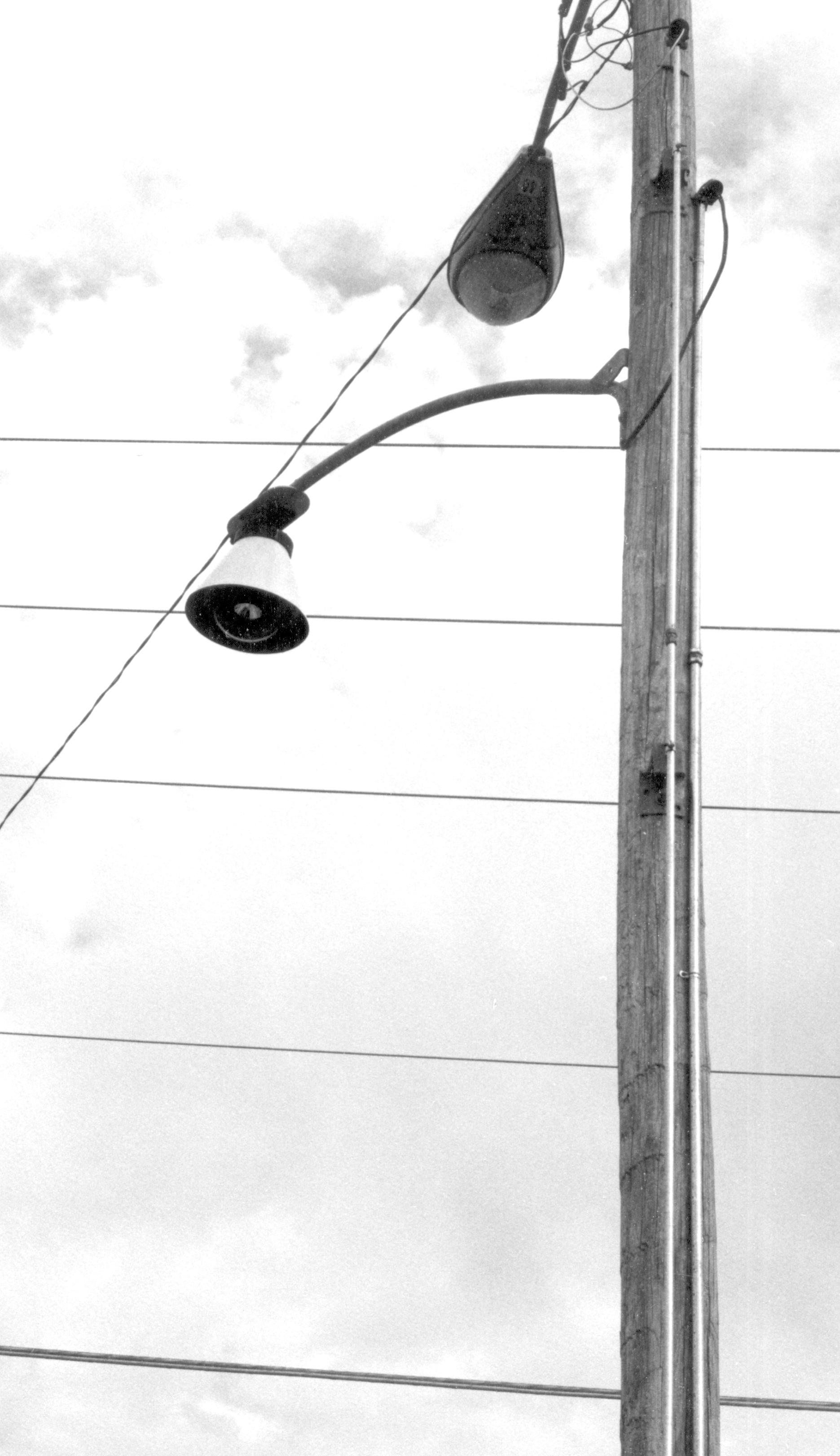
At the roundabout, the camera was installed on an existing street light pole in the southeast corner of the intersection. The camera was attached to the end of a street light arm that was then attached to the wood street light pole. The camera was mounted perpendicular to the ground, which allowed the video image to be relatively distortion free to the horizon in all directions. The camera was mounted similarly for data collection at the two non-roundabout locations.
Mounting heights for the camera were approximately 6 meters (20 feet) above the street surface. According to the manufacturer specifications, this mounting height provides a focal plane of approximately 40.5 meters by 54.0 meters (133 feet by 177 feet) (List). The camera allows the focal plane to be changed (made larger or smaller) based on the height above the intersection. The camera was generally mounted directly above the curbline; however, this was strictly a function of field conditions (pole location).
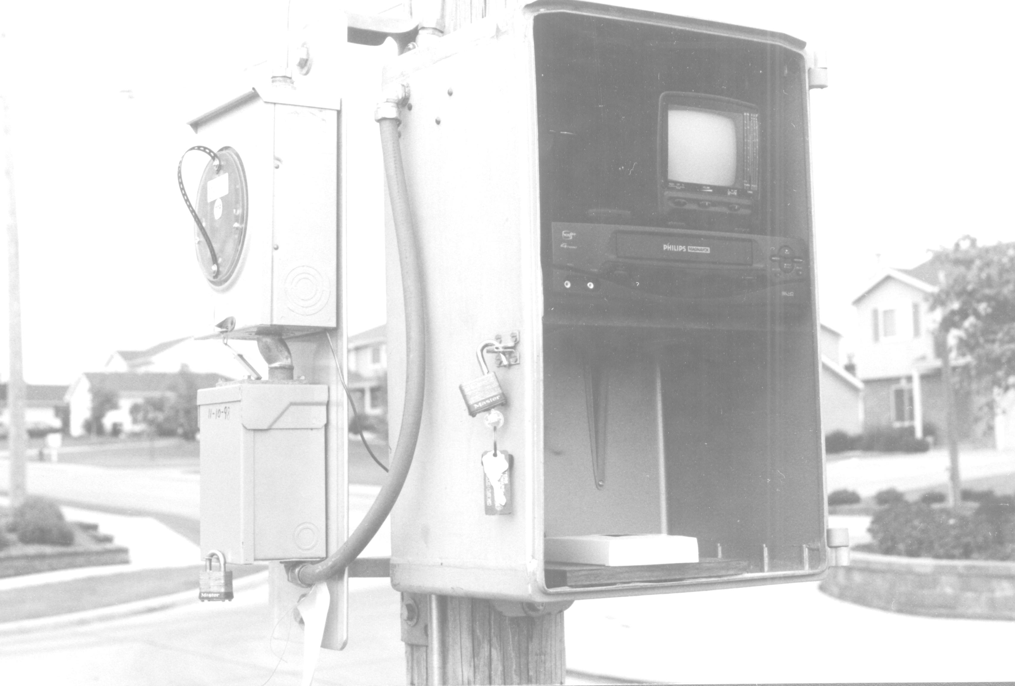
At all intersections the camera feed went into a VCR/ TV unit housed in a recycled traffic signal controller cabinet (see Figure 7). This allowed all equipment to be mounted on a single pole. The signal cabinet provided a secure weather tight location for the recording equipment.
The video image was recorded on standard VHS videotapes. This required site visits each time a new tape was needed. In all, over 200 hours of videotape was collected from the three intersections.
The reason for video data collection was used was two-fold. First, it allowed data to be collected for examination at a later time. Second, the videotape could be viewed and re-viewed during the data analysis phase of the project. This method was used on a study in New York (6).
"Information on volumes, lane usage, and delays were extracted from the resulting video tapes to learn more about how automated data extraction schemes might be devised and to perform capacity analysis…. Second, it seemed that the use of an omnidirectional camera at roundabouts might be a very cost-effective instrumentation option. Instead of either an array of pavement-based sensors, or a collection of conventional camera, a single omnidirectional camera, strategically placed, could provide information about all movements at the facility simultaneously" (6).
Similar to these findings, the ability to have the videotapes of the intersection in operation was invaluable through this research.
SECTION 3.2 – Manual Data Collection
Manual data collection refers to the manual extraction of data from the videotapes. Once the videotapes were collected, they were evaluated through observation. The two objectives of the manual data collection were to obtain traffic flows and traffic conflicts.
Traffic flows were observed on the tape and the information (turning movement counts) recorded on pre-prepared data sheets. The traffic counts were recorded in 15-minute intervals, which became the input information for analysis by the computer program SIDRA.
The second type of data collected by videotape observation was traffic conflicts.
"A traffic conflict is a traffic event involving two or more road users, in which one user performs some atypical or unusual action, such as a change in direction or speed, that places another user in jeopardy of a collision unless an evasive maneuver is undertaken" (7).
Traffic conflicts are discussed in detail in a later chapter on safety. Each tape reviewer was trained on the types of traffic conflicts and how to identify them. The tape reviewers watched for traffic conflicts as they collected the traffic flow data.
SECTION 3.3 – Comparable Intersections
The Manhattan roundabout was constructed prior to the initiation of this study. Therefore, the before/ after method of evaluating its operation was not available to the research team. Instead, evaluation was performed by comparing the operation of the roundabout to two comparable intersections.
A comparable intersection was determined to be one that had the same general physical layout, and operated under similar traffic loadings as the roundabout. Comparable locations were geographically limited to the City of Manhattan, Kansas. This was due to the field support provided by the City and the desire to have all intersections located within the City. Having all intersections located within the City allowed the creation of public awareness information where all information and conclusions stem from a single jurisdiction. It also avoids the possible differences that could be present if drivers from different locals were examined.
The general physical and operational features of the roundabout, and those desired of the comparable intersections, were determined to be as shown in Table 5. These traits were used to select a set of possible comparable intersections from all possible locations within the corporate limits of the city of Manhattan, Kansas. The criteria were established to guide selection toward locations that would operate similarly to the Candlewood/ Gary intersection had the roundabout not been constructed. In this way, inferences could be made following experimentation as to weather the operation of the roundabout was better, worse, or similar to more traditional intersection traffic controls.
The study team and advisory committee members reviewed the possible comparable intersections. Based on personal knowledge of the intersections and study focus, two comparable intersections were chosen.
One comparable intersection was located at Dickens Avenue and Wreath Avenue (DW). This 4-leg intersection is located on the west side of Manhattan. Both roads were 2-lane collector roads carrying traffic levels at those specified in the selection criteria. Posted speed limits on both streets were within the range specified. This intersection operated under two-way STOP control.
TABLE 5 - Comparable Intersection Selection Criteria
|
Physical Traits:
|
General Description/ Range:
|
| Approach legs |
Four |
| Number of approach lanes |
One* |
| Type of approach roads |
Local and/or collector |
| Total intersection traffic volume |
5,000 – 10,000 vpd |
| Approach speeds |
40 – 56 kph (25 – 35 mph) |
*Had the Candlewood Drive/ Gary Avenue roundabout not been built, turn lanes would most likely have been striped to accommodate turning movements. Therefore, the number of approach lane criteria relates to thru lanes only.
The second comparable intersection chosen for study was located at Juliette Avenue and Pierre Street (JP). This was the intersection of a 2-lane collector and a 2-lane local road. Traffic levels and speeds on both streets fell within the trait range specified. This intersection operated under two-way STOP control.
SECTION 3.4 – Data Analysis
This phase of the project began with a statistical evaluation of raw traffic data to assure that the three intersections were being observed under ‘similar’ traffic conditions. Then the data was used as input into the computer evaluation program SIDRA. This software was used to evaluate all three intersections operating under their existing traffic control (roundabout, two-way STOP). SIDRA provided output values for the six measures of effectiveness (MOEs) (described in Table 6). This data was then statistically evaluated to determine which, if any, of the three intersections could be considered to be operating better then the others.
TABLE 6 - Intersection Measures of Effectiveness
|
Measure of Effectiveness:
|
Description:
|
| 95% Queue |
Length of the queue for all approaches at the 95% confidence level |
| Average Delay |
Average vehicle delay for all entering vehicles |
| Maximum Approach Delay |
Average vehicle delay for the approach with the highest average vehicle delay |
| Proportion Stopped |
Proportion of entering vehicles that are required to stop due to vehicles already in the intersection |
| Maximum Proportion Stopped |
Proportion of entering vehicles that are required to stop due to vehicles already in the intersection on the approach with the highest proportion stopped value |
| Degree of Saturation |
Amount of capacity that is consumed by the current traffic loading (commonly referred to as the v/c ratio) |
The study MOEs initially included Level of Service (LOS). This MOE was dropped as it was found that the three intersections operated at LOS A/B (8). The narrow range of LOS values did not allow meaningful analysis based on level of service values to be completed. Since LOS is based on average vehicle delay, the LOS analysis was not lost, simply replaced by the more precise measure of average vehicle delay.
The intersection MOEs were compared with one another using standard statistical methods. Testing for normality and equal variances was performed first. This was followed by one of three statistical tests, depending on the results of the normality and equal variance testing. Conclusions were drawn for each MOE with regard to the operation of the intersections and intersection control types.
This study was designed to evaluate the operation of the roundabout in Manhattan, Kansas. The conclusions from this study will apply to other locals only if the overall conditions are similar to that found in this study. If the conditions in other places differ significantly from those found here, detailed local study is warranted. Such detailed study could use the same procedures developed here with the use of local data. In all cases, the results of this study provide additional information for use throughout the United States with regard to increasing the roundabout knowledge database.
Before and after operational data was not available at the Candlewood Drive/ Gary Avenue (CG) intersection. Other similar intersections were used to compare with the roundabout.
SECTION 4.1 – Dickens Avenue/Wreath Avenue (DW)
The intersection of Dickens Avenue and Wreath Avenue (DW) is the junction of two collector roads. The adjacent land use consists of residential in both south quadrants, a regional park in the northwest quadrant, and a vocational school in the northeast quadrant.
Traffic volumes on the approach legs were found to be similar to that at the roundabout intersection. Typical traffic levels at this intersection are shown in Table 7. The approach volumes ranged from 1,354 to 2,770 on a daily basis. The intersection approach totals are shown graphed in Figure 8. During the AM and PM peak hours, the intersection carried 615 and 680 vehicles respectively. These traffic counts were collected on Tuesday, April 20, 1999.
Vehicle speed data was also collected on the approaches to this intersection. The approach speeds ranged from 35 to 51 kph (22 to 32 mph) (see Table 8).
The two roads are both two-lane with one lane in each direction. Parking is restricted near the intersection allowing creation of a turn lane on each approach. The north and south approaches have one left turn lane and a combined thru/ right lane. The east and west approaches have combined left/ thru lane and a separate right turn lane. The east and west approaches are STOP sign controlled while the north and south are not controlled.
While the west approach road drops away from the intersection, the intersection and approach are essentially level.
TABLE 7 - Dickens Avenue/ Wreath Avenue Approach Traffic Counts
FIGURE 8 - Dickens Avenue/ Wreath Avenue – Total Approach Traffic Counts
TABLE 8 - Dickens Avenue/Wreath Avenue 85 Percentile Approach Speeds
|
Approach
|
North |
South |
East |
West |
| 85% Speed (kph) |
41 |
36 |
52 |
49 |
| (mph) |
25 |
22 |
32 |
30 |
The 22 data traffic counts for the Dickens Avenue/Wreath Avenue intersection are shown in Table 9. This table also shows the corresponding peak hour factor and the resulting maximum hourly flow. Initial statistical analysis looked at whether the data was normally distributed. The cumulative frequency histogram of the raw traffic counts in shown in Figure 9. The data in this figure appears to follow the standard normal curve shape for a normal distribution.
TABLE 9 - Dickens Avenue/Wreath Avenue Traffic Count Data
|
Date:
|
Day of Week:
|
Count:
|
Peak Hour Factor:
|
Max Peak Hour:
|
| 5/7/99 |
Friday |
215 |
0.53 |
406 |
| 4/22/99 |
Thursday |
258 |
0.85 |
304 |
| 5/7/99 |
Friday |
263 |
0.85 |
309 |
| 5/7/99 |
Friday |
269 |
0.87 |
309 |
| 4/21/99 |
Wednesday |
270 |
0.84 |
321 |
| 4/22/99 |
Thursday |
291 |
0.84 |
346 |
| 5/4/99 |
Tuesday |
293 |
0.94 |
312 |
| 5/6/99 |
Thursday |
306 |
0.90 |
340 |
| 5/5/99 |
Wednesday |
307 |
0.83 |
370 |
| 4/22/99 |
Thursday |
310 |
0.91 |
341 |
| 4/21/99 |
Wednesday |
310 |
0.86 |
360 |
| 5/3/99 |
Monday |
323 |
0.49 |
659 |
| 5/6/99 |
Thursday |
325 |
0.71 |
458 |
| 4/23/99 |
Friday |
353 |
0.64 |
552 |
| 5/3/99 |
Monday |
414 |
0.62 |
668 |
| 5/6/99 |
Thursday |
415 |
0.86 |
483 |
| 4/22/99 |
Thursday |
437 |
0.87 |
502 |
| 5/7/99 |
Friday |
440 |
0.74 |
595 |
| 5/5/99 |
Wednesday |
447 |
0.67 |
667 |
| 5/6/99 |
Thursday |
466 |
0.71 |
656 |
| 4/22/99 |
Thursday |
479 |
0.77 |
622 |
| 5/5/99 |
Wednesday |
480 |
0.77 |
623 |
| |
|
340
|
0.77
|
444
|
|
Summary:
|
| |
Max: |
480 |
Range: |
265 |
| |
Min: |
215 |
|
|
FIGURE 9 - Cumulative Frequency Distribution of Traffic Counts - DW
SECTION 4.2 – Juliette Avenue/Pierre Street (JP)
The intersection of Juliette Avenue and Pierre Street (JP) is located south of the downtown in Manhattan, Kansas. Juliette Avenue is a north/ south collector road and Pierre Street is an east/ west local street. The adjacent neighborhood land use is primarily residential.
Traffic volumes on the approach legs were found to be as shown in Table 10. The daily approach volumes ranged from 1,106 to 3,660 vehicles. The intersection approach totals are shown graphed in Figure 10. During the AM and PM peak hours, the intersection carried 641 and 1,040 vehicles respectively. These traffic volumes were collected on Tuesday, May 11, 1999.
Vehicle speed data on the approaches to the intersection ranged from 54 to 62 kph (33 to 38 mph) (see Table 10).
TABLE 10 - Juliette Avenue/Pierre Street Approach Traffic Counts
FIGURE 10 - Juliette Avenue/Pierre Street – Total Approach Traffic Counts
The two intersecting streets are both two-lanes with one lane in each direction. Parking is restricted near the intersection. No specific turn lanes are marked on the street; however, during times of heavy traffic, informal turn lanes develop. The east and west approaches are STOP sign controlled while the north and south are not controlled.
The intersection is level on all approaches.
Traffic volumes for this intersection for each of the study hours are shown in Table 12. An examination of the cumulative frequency histogram (see Figure 11) showed that the raw traffic count data exhibited the approximate shape of normally distributed data.
TABLE 12 - Juliette Avenue/Pierre Streeet Traffic Count Data
|
Date:
|
Day of Week:
|
Count:
|
Peak Hour Factor:
|
Max Peak Hour:
|
| 8/28/99 |
Saturday |
206 |
0.79 |
261 |
| 8/22/99 |
Sunday |
236 |
0.89 |
265 |
| 8/17/99 |
Tuesday |
242 |
0.85 |
285 |
| 8/22/99 |
Sunday |
270 |
0.96 |
281 |
| 8/17/99 |
Tuesday |
303 |
0.88 |
344 |
| 8/23/99 |
Monday |
304 |
0.67 |
454 |
| 8/28/99 |
Saturday |
305 |
0.88 |
347 |
| 8/23/99 |
Monday |
307 |
0.94 |
327 |
| 8/17/99 |
Tuesday |
311 |
0.80 |
389 |
| 8/25/99 |
Wednesday |
315 |
0.55 |
573 |
| 8/25/99 |
Wednesday |
317 |
0.89 |
356 |
| 8/22/99 |
Sunday |
320 |
0.86 |
372 |
| 8/16/99 |
Monday |
328 |
0.66 |
497 |
| 8/25/99 |
Wednesday |
329 |
0.89 |
370 |
| 8/16/99 |
Monday |
353 |
0.95 |
372 |
| 8/23/99 |
Monday |
370 |
0.84 |
440 |
| 8/17/99 |
Tuesday |
378 |
0.66 |
573 |
| 8/17/99 |
Tuesday |
389 |
0.91 |
427 |
| 8/16/99 |
Monday |
416 |
0.85 |
489 |
| 8/28/99 |
Saturday |
426 |
0.87 |
490 |
| 8/28/99 |
Saturday |
437 |
0.93 |
470 |
| 8/25/99 |
Wednesday |
495 |
0.91 |
544 |
| |
|
328
|
0.83
|
395
|
| Summary: |
| |
Max: |
495 |
Range: |
289 |
| |
Min: |
206 |
|
|
FIGURE 11 - Cumulative Frequency Distribution - Juliette Avenue/Pierre Street
SECTION 4.3 – Comparison of Traffic Volumes at the Three Study Intersections
Three intersections carrying three similar, but different levels of traffic were evaluated. To determine when the hourly traffic data was to be collected at each, ‘study hours’ were determined. At the roundabout (CG), the study hours represented times of maximum traffic flow. Maximum traffic flow was chosen as the literature indicated that the hourly traffic range carried by the Manhattan roundabout was at the low end of the scale for existing roundabouts in the United States (as shown in Figure 2). Also, using maximum traffic flow would allow examination of the roundabout under peak loading conditions. These traffic volumes ranged from 224 to 402 vph and averaged 310 vph.
The peak traffic levels carried at the two comparable intersections were much higher than those found at the roundabout. Therefore, data was collected at the two comparable intersections (DW and JP) during times when the traffic at these intersections was near the range of the roundabout traffic volumes. Referring to Figure 12, the peaks for the roundabout (CG) intersection occur near 8:00 AM and from 4:00 – 7:00 PM. To achieve similar traffic volumes as occurred at the roundabout, the Dickens Avenue/ Wreath Avenue intersection was studied in general at 7:00 AM and from 7:00 – 9:00 PM. Similarly, the Juliette Avenue/ Pierre Street intersection was examined during the periods around 7:00 AM, 3:00 PM and after 7:00 PM. These non-peak times at the comparable STOP controlled intersection resulted in hourly traffic counts at DW that ranged from 263 to 480 vph and averaged 340 vph. At JP, the values ranged from 206 to 495 vph and averaged 238 vph. This method of selective data collection allowed the thre intersections to be evaluated under comparable traffic conditions as required in the study design.
FIGURE 12 - Comparison of Entering Volumes at the Three Study Intersections
Safety benefits are touted by many as an advantage of a roundabout (1, 2, 4, 9, 10, 11, and 12). This study examined the issue of intersection safety in three ways: literature review, conflict analysis and crash review.
SECTION 5.1 – Literature Review
There were a number of safety and operational concerns expressed by citizens to the City staff prior to the construction of the Candlewood/ Gary roundabout. There were also a number of consistent issues raised in the literature with regard to roundabout safety and operation. Since the local safety concerns paralleled those found in the literature, they are presented here together (Table 13).
TABLE 13 - Safety and Operational Concerns of Roundabouts
|
Concern:
|
Description at a Standard Intersection:
|
Description at a Roundabout:
|
| Non-compliance |
Drivers not obeying traffic control devices |
Drivers driving the wrong way around roundabout |
| Truck accessibility |
Can trucks maneuver past curbs |
Can trucks maneuver around the center island |
SECTION 5.1.1 - Safety of Roundabouts
Previous studies of crash experience finds that roundabouts are safer than standard methods of intersection control. The following are examples of results from such studies:
- A 1975 study found that intersections where roundabouts had replaced standard major/ minor controls resulted in 39% fewer injury crashes, 64% less serious injury and fatal crashes, 51% fewer wet road crashes, and 46% fewer pedestrian crashes (13).
- A 1994 study found that annually 22.40 crashes occurred at three roundabouts producing 4.26 injuries. Three adjacent two-way STOP controlled intersections experienced 48.75 crashes producing 19.73 injuries per year. The STOP controlled intersections were found to have a crash rate almost double the roundabout intersections, 1.22 versus 2.41 (12).
- A 1998 study reports that where roundabouts have been installed in the United States, there has been a reduction in the number of property damage only crashes of from 10 to 32 percent, a reduction in injury crashes of from 31 to 73 percent and a reduction in fatal crashes of from 29 to 51 percent (5).
Overall, the findings of safety may be best stated by Wallwork, "The safest, most efficient and attractive form of traffic control in the world" (2). There is documented evidence to support the claim that roundabouts are a safe intersection control.
The safety benefits of roundabouts may be a result of simplifying the driving task. At a standard intersection, the driver is required to react to vehicles to the right, left, and ahead, and to pedestrians on all parts of the intersection. "The apparent reason for safety benefits of traffic circles are that the motorists, bicycles and pedestrians are required to check for traffic from only one direction at a time, thereby simplifying the task" (12). The term ‘traffic circles’ used by Savage describes what is referred to in this research as a roundabout.
SECTION 5.1.2 - Bicycle and Pedestrian Safety
There were safety issues raised prior to the roundabout being installed with regard to access for pedestrians and bicyclists. This fear appeared to stem from the unfamiliarity of the residents to the intersection design. Upon examination of the literature (4, 5), it does appear that the operation of bicyclists and pedestrians through roundabouts is an issue that needs to be carefully considered.
Savage (12) found that roundabout intersections experienced less bicycle and pedestrian crashes than adjacent two-way STOP controlled intersections. Specifically, the roundabout intersections had a crash rate of 0.06 crashes per million vehicles for bicycle and pedestrian involved crashes. This compared to a crash rate of 0.27 for the two-way STOP controlled intersections. Other sources present similar findings (2, 10). Based on the published literature, properly designed roundabouts provide a safe environment for bicyclists and pedestrians (2).
SECTION 5.1.3 - Bicycle and Pedestrian Design
The physical design of a roundabout for bicyclists and pedestrians must be examined separately by mode.
Bicyclists can negotiate a roundabout as either a vehicle or pedestrian. Bicyclists that feel comfortable with travelling in the traffic stream can continue into the roundabout using the same path as vehicles. The Maryland roundabout design guide states that "cyclists use roundabouts in a similar manner to motor vehicles" (1). The other option for a bicyclist is to leave the street and travel on the sidewalk system. One suggestion for addressing these users is to install a bicycle ramp that transitions from the street bike lane to the sidewalk for these bicyclists (Wallwork).
Pedestrian design of roundabouts follows a design philosophy similar to standard intersections.
"In respect to geometric design, the provision for pedestrians does not differ greatly to that required for other intersection treatments, however, certain roundabout designs, particularly large roundabouts, can result in greater walking distances, and thus inconvenience, of pedestrians" (3).
In general, pedestrian crossings (crosswalks) should be located one vehicle length back from the entrances and exits of the roundabout (1, 2). When crossing volumes of pedestrians are high, it may be desirable to move the crosswalk location farther back from the entrance/ exit to allow both the motorist and pedestrian a chance to see each other away from the activities of the roundabout (2). In addition to the location of the crosswalk, a properly designed splitter island is important to pedestrian safety.
"Generally, the installation of well designed splitter islands of sufficient size to stage pedestrians, thus allowing them to cross only one direction of traffic at a time, will result in pedestrians being able to move more safely and freely around the intersection than was the case before the installation of the roundabout" (3).
In all cases, the splitter island plays a vital role to the safe movement of pedestrians and beginner bicyclists through a roundabout intersection.
SECTION 5.2 – Crash Review
Full year crash data was available from the City for the Candlewood Drive/ Gary Avenue intersection for the calendar years 1994 – 1996 prior to installation of the roundabout, and for 1998 - 1999 after installation. The number and type of intersection crash are shown in Table 14. While complete year data is not available, data was available for 29 months following roundabout construction. This ‘after’ data shows no reported traffic crashes at this intersection. This represents a statistically significant reduction in crash experience based on the methodology in the Kansas High Accident Location Manual (14).
TABLE 14 - Crash Records Before and After Roundabout Installation
|
Year:
|
PDO:
|
Injury:
|
Total:
|
| 1994 |
3 |
0 |
3 |
| 1995 |
0 |
2 |
2 |
| 1996 |
2 |
2 |
4 |
| Roundabout Installed in 1997 |
| 1998 |
0 |
0 |
0 |
| 1999 |
0 |
0 |
0 |
* PDO – Property Damage Only
There were nine reported crashes at the intersection of Candlewood Drive/ Gary Avenue from January 1994 to December 1996. All nine of these crashes involved a driver failing to yield the right of way or failing to stop for a STOP sign. All of the nine crashes were right angle. The literature indicates that right angle and failure to yield type crashes are the types that are reduced by installation of a roundabout as was found to be the case at the Manhattan roundabout.
The Manhattan roundabout experienced no reported crashes in 29 months of operation. The before condition experienced nine crashes over 3 years, 4 of which involved injuries. Using Kansas’s HAL procedure (14) for calculating the cost of crashes yielded the values shown in Table 15. This table shows that the Manhattan roundabout has reduced the annual cost to society from vehicle crashes by $87,833. All amounts are in non-adjusted, 1994 dollars.
TABLE 15 - Before and After Crash Costs at Roundabout
| |
Before
|
After
|
| PDO Crashes @ $3,500 ea |
5 x $3,500 = $17,500 |
0 x $3,500 = $0 |
| Injury Crashes @ $61,500 ea |
4 x $61,500 = $246,000 |
0 x $61,500 = $0 |
| Total Cost of Crashes |
$263,500 |
$0 |
| Time Period |
3 years |
2 years |
| Crash Cost per Year |
$87,833 |
$0 |
The monetary values in this table are not adjusted for inflation.
SECTION 5.4 – Conflict Analysis – Literature Review
Intersection crashes are statistically rare events. It usually takes several years of crash data to make valid conclusions. As such, techniques have been developed to predict the relative safety of an intersection in the absence of sufficient crash data. This study used the conflict analysis technique to evaluate the safety of the three intersections under analysis.
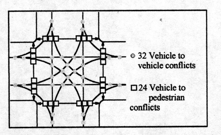
One of the observational methods of determining the possible danger of an intersection configuration is to examine the number of conflict points (2, 7). By definition, a conflict point is any point where a vehicle path crosses, merges, or diverges from another vehicle or pedestrian path. As can be seen in Figure 13, a standard 4-leg intersection has 32 vehicle and 24 pedestrian conflict points. Figure 14 shows the conflicts for a roundabout. Note that a roundabout decreases the number of vehicle and pedestrian conflict points to eight each. Also note that for the roundabout, all left turn and crossing conflict points are alleviated. Theoretically, the roundabout should operate much safer than a standard intersection.
FIGURE 13 – Standard Intersection Conflict Points
Source: (2)
FIGURE 14 - Roundabout Intersection Conflict Points
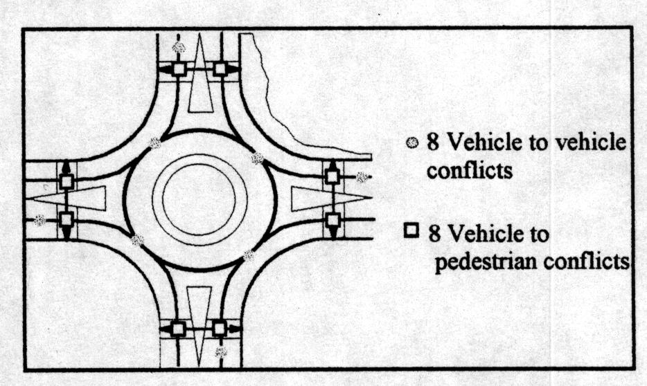
Source: (2)
The definition of a traffic conflict leads to a sense that the traffic conflict is a measure of operational break points of the intersection being observed. Indeed, the reference states that this method of intersection analysis is "useful in diagnosing problem locations or measuring the effectiveness of a site improvement" (7). As used in this study, the traffic conflict analysis measured the comparative operation of multiple intersections, and the results of that analysis. The results of the conflict analysis were used to make conclusions regarding safety of the roundabout under study.
Intuitive understanding of how a roundabout may be safer than a standard intersection lies in comparison of the conflict point diagrams. Another lies in examining the tasks placed on drivers as they pass through each type of intersection. To pass through a traditionally controlled intersection, a driver, must look for approaching/ conflicting vehicles to the left and right, as well as watch the opposing direction for vehicles that may turn into his/her path. Once a check for pedestrians is made, traversing a roundabout requires the driver to watch traffic only from the left. Therefore, the observational tasks placed on a driver at a standard intersection are much greater than they are at a roundabout intersection.
In NCHRP report number 219 (7), thirteen basic intersection traffic conflicts are defined, arising from the 32 vehicle/ vehicle intersection conflict points (Table 16). Also shown are how these typical intersection conflicts apply to an intersection configured under roundabout control. This table shows that by using a roundabout at an intersection, all but three of the 13 basic intersection conflicts are alleviated.
In one sense, the roundabout tends to be both a geometric design feature, and a traffic control device. The roundabout affects the speed of vehicles traveling through the intersection by its design components. The roundabout also provides for a logical yield control of vehicles at the intersection. In many cases however, roundabouts are considered an alternative where traffic signalization is needed. Therefore, the primary consideration of the roundabout is as a traffic control device.
TABLE 16 - Basic Intersection Conflicts - Standard Intersection and Roundabout Control
|
Conflict Type
|
Standard Intersection*
|
Roundabout
|
- Left turn, same direction
|
Yes |
No |
|
|
- Right turn, same direction
|
Yes |
Yes |
| Slow vehicle, same direction |
Yes |
Yes |
| Lane Change |
No |
No |
| Opposing left turn |
Yes |
No |
| Right turn cross traffic, from right |
Yes |
Yes |
| Left turn cross traffic, from right |
Yes |
No |
| Thru cross traffic, from right |
Yes |
No |
| Right turn cross traffic, from left |
Yes |
No |
| Left turn cross traffic, from left |
Yes |
No |
| Thru cross traffic, from left |
Yes |
No |
| Opposing right turn on red (during protected left turn phase) |
Yes |
No |
Pedestrian
|
Yes |
Yes |
| Total: |
12 |
3 |
* Standard intersections include YIELD, STOP and signal control
SECTION 5.5 – Conflict Analysis – CG, DW and JP
Many of the tapes were reviewed by members of the study team for the presence of conflicts. Despite these efforts, and the observation of over 180 hours of videotapes, only one conflict was observed. The one conflict occurred at one of the two-way STOP controlled intersections. Due to the insufficient number of observed conflicts, conflict conclusions could not be made.
SECTION 5.5 – Intersection Travel Speed
The speed at which a vehicle travels through an intersection can have a great impact on the severity of any crash that may occur. The intersection travel speed can even have an impact on the number of intersection crashes. This is due to the shorter decision times allowed to motorists (and non-motorists) when vehicles operate through a high speed intersection. Therefore, any intersection design feature that would tend to consistently slow vehicles would have a positive impact on safety. Roundabouts through their design (splitter islands, deflection curve) slow vehicles down.
SECTION 5.6 – Summary of Safety Evaluation
The literature contains clear evidence that roundabouts are safer than other forms of intersection traffic control. Safety benefits were found to apply to all intersection users including vehicles, pedestrians and bicyclists.
There were nine reported vehicle crashes in the three calendar years preceding roundabout installation at the intersection of Candlewood Drive/ Gary Avenue. These nine crashes were all right angle and involved a driver railing to yield right of way at the STOP controlled intersection. There were no reported vehicle crashes in 29 months after roundabout installation. This reduction in crashes was found to be statistically significant at the 95% confidence level. This reduction in right angle/ failure to yield crashes matches the safety benefits of roundabouts suggested by the literature.
The reduction in crashes from an average of three per year to zero resulted in a savings to society of crash costs.
An examination of traffic conflicts was performed at all three intersections (CG, DW and JP). Insufficient data was obtained from the conflict study to perform analysis or make conclusions with regard to intersection conflicts.
Overall, the safety of the Manhattan roundabout has been as predicted by the literature. This may suggest that safety at U.S. roundabouts may be similar to other countries where they are in use. However, there is relatively limited data from U.S. roundabouts, requiring researchers and practitioners to supplement their findings with foreign safety studies. Additional data regarding of the safety of U.S. roundabouts will accrue as more and more are built.
This study examined the operation of three intersections under similar traffic loadings. The data used to evaluate intersection operation was based on traffic counts. To assure that the three intersections were examined under similar loadings, comparable study hours were used instead of the more typical peak hours.
SECTION 6.1 – Daily Traffic Volumes
The process of gathering hourly traffic volumes began with an examination of the daily traffic at the three intersections under examination. Daily traffic counts were collected on the approach roads to each intersection. The approach counts were then examined to see when the traffic levels at the three intersections would be the same. This approach resulted in the study team using the terminology ‘study hours’ rather than the more typical ‘peak hours’. This process was explained in Chapters 2 and 3.
The initial statistical analysis centered on whether the hourly volumes for the three intersections could be considered to have come from the same population. If not, then the intersections could not be said to be operating under similar traffic conditions and the study design would be invalid. If the volumes were found to be similar, the data could be considered to be from one population and further analysis could be conducted. Two sets of count data were analyzed: raw traffic counts and SIDRA calculated traffic counts.
The raw traffic counts were those that were collected from the videotapes. These represent field measurements of the actual traffic flows. The SIDRA traffic counts are those that are calculated internally within the computer program from the raw counts. These counts are obtained by using equation 6.1.
VolSIDRA = Volhour / Peak Hour Factor (6.1)
The null hypothesis for testing both the raw and SIDRA traffic counts was that the three intersection count means were equal (see equation 6.2). This hypothesis was evaluated using the analysis of variance F-test. For the raw traffic counts, the resulting p-value was 0.2058. This p-value is greater than the stated alpha value of 0.05, which results in the test failing to reject the null hypothesis. The raw counts can therefore be considered to have come from the same population and the intersections can be said to be operating under similar conditions.
Ho: m CG = m DW = m JP, a = 0.05 (6.2)
Section 8.1 presents the results of the statistical testing on the SIDRA traffic count data showing that the three sets of data came from the same population.
SECTION 6.2 – Intersection Delay
Vehicles operating through an intersection experience two distinctive types of delay: geometric and queuing (3). Total vehicle delay is the sum of both types of delay.
Geometric delays are defined as those delays encountered during travel through the intersection. Geometric delays are measured as the time it takes a vehicle to traverse the intersection from entry point to exit point. It may be appropriate to include these delays in a cost analyses to account for the extra time it may take vehicles to travel around the middle island of a roundabout (13). Geometric delays are highest for left turn maneuvers where a vehicle must travel around the central island of a roundabout. U-turns are not included here as they are not possible at most non-roundabout intersections).
The other type of delay is operational. This is the delay that occurs when entering vehicles are delayed by the presence of vehicles already in the intersection. A 1994 report presented the operational delays through intersections under roundabout control and comparable two-way STOP controlled intersection using the NETwork SIMulation (NETSIM) computer method. The results of the comparison found that roundabouts operated better (less delays, stops, and higher average speed) than the best two-way STOP controlled intersection. In conclusion, "(t)he study also shows that the measures of effectiveness can be improved by converting the two-way stop intersections to traffic circles" (12). The Savage study dealt with a physical intersection design for roundabouts, not traffic circles as currently defined.
A New York study of intersection operations found the following behaviors present at roundabouts:
"Delays occur at the exits as well as the entrances, with weaving movements taking place between vehicles leaving the roundabout and those entering just upstream…. It is common to have an upstream exit affect a downstream entry…. It is unusual to have a downstream entry affect an upstream one" (6).
The New York study observations were possible through the use of an omnidirectional camera that could video all approaches at once as was done in this study.
SECTION 6.3 - Delay at the Manhattan Roundabout
Vehicle Delay was one of the measures of effectiveness used in the study of the Manhattan roundabout. This value was not measured directly in the field, or from the video collected for data purposes, but was obtained from calculated computer output of operation at the roundabout.
Hourly count data was input into SIDRA where one of the outputs was vehicle delay. SIDRA provided average vehicle delay by approach and for the entire intersection. Vehicle delay was examined in two ways.
Overall intersection average delay represents the total delay experienced by all entering vehicles divided by the total number of entering vehicles. This value is commonly used to generate an intersection level of service (LOS) value. LOS was not used in this study because all hour periods evaluated were found to operate at LOS ‘A’ at the intersection level and most approaches operated at the LOS ‘A’ level with the remaining operating at LOS ‘B’. Average vehicle delay was used as it provides a more precise measure of intersection operation than LOS.
Use of the SIDRA (version 5.20b) computer program allowed the comparison of the roundabout and traditional intersections under a number of varying traffic flow and control conditions.
Other researchers have performed computer analysis of operation of roundabouts. Savage (1994) reported on a comparison of capacities for roundabouts versus two-way STOP controlled intersections (12). The evaluation used the Highway Capacity Manual (HCM) (8) for determining operations at the STOP controlled intersections and a method developed by Troutbeck for the roundabouts. In all cases, operation of the roundabouts was better than the two-way STOP controlled intersections under similar traffic conditions (12).
SIDRA was used to evaluate the operation at the Candlewood Drive/ Gary Avenue roundabout. This model evaluates the operation using gap acceptance theories accepted by the Australian Road Authority and similar to those adopted for use by the HCM software. Competing computer models (RODEL and ARCADY) both use British empirical formulas for evaluating roundabout operation. There is some question as to the validity of the gap acceptance model at near capacity conditions (defined by SIDRA as v/c ³ 0.85). Since this study examined a low volume roundabout, the capacity issues surrounding gap acceptance theory near capacity do not apply.
SIDRA was installed to operate on the HCM methodology with vehicles driving on the right. The SIDRA software allows the user to choose the side of the road the traffic drives on as it is used throughout the world. Queue lengths were calculated using a vehicle length of 7.6 meters (25 feet). The Candlewood Drive/ Gary Avenue geometric features required for SIDRA were based on measurements taken from the construction plans. Sample results of the SIDRA analysis of the roundabout are provided in Appendices 3, 4 and 5. While SIDRA can provide a number of output measures, only those output values relating to the study measures of effectiveness are included in this report.
Using standard statistical techniques (15, 16), the output data from the SIDRA model was analyzed to determine how the operation of the roundabout (CG) compared to that of the two comparable two-way STOP controlled intersections (DW and JP). Twenty-two data points (hourly traffic counts) were available for each location. SIDRA provided data for each of six measures of effectiveness (MOEs). The statistical analysis of each MOE is presented individually in the following sections of the report.
SIDRA output for all sixty-six hourly traffic counts were evaluated using SAS. The statistical tests were performed using the Statistical Analysis Software (SAS) version 6.12 on the Kansas State University Unix operating system.
Two base assumptions exist for the use of most statistical tests: normality and equal variances. These two data assumptions were tested prior to determining what specific statistical test to use to evaluate the intersection operation as it related to the MOEs. The statistical process is summarized in Table 17.
The first test of normality was an evaluation of the relationship between the interquartile range and the standard deviation. The interquartile range is the difference between the 25th and 75th percentile values and was obtained from the SAS computer output. Similarly, the standard deviation for each data set was obtained from the SAS output. A normal distribution was indicated if the ratio of these two values was near 1.3. For the purposes of this study, this normality indicator was satisfied if the IQR/S value was within +/- 50% of the desired 1.3 value.
The Shapiro-Wilk test was also used for evaluating normality. This test is sensitive to small samples. To lessen the possibility of a false rejection, a small alpha value of 0.01 was chosen.
The determination of normality was based on the results of both tests. While in most cases, the results were similar (either showing normal or not normal); there was a range in the individual test results. Therefore, the normal determination was a judgement decision based on the two test results. Normality is identified as test ‘I’ in the MOE statistical tables.
The second area to be examined was that of equal variances. Equal variances between the three data sets were tested using the Levene’s test. This test is sensitive to normality assumptions; therefore, the null hypothesis was rejected only if the test p-value was less than 0.01 (a value). The equal variance test is identified as ‘II’ in the statistical summary tables.
One of three different statistical paths were chosen based on the results of the normality and equal variance tests (see tests III.A, IIIB and IIIC in Table 17).
If the data was found to be normally distributed with equal variances, the equality of the means was tested using the analysis of variance (ANOVA), F-test. An alpha value of 0.05 was used for this test. If the analysis of variance test resulted in a failure to reject the null hypothesis, then the statistical process stopped. Failure to reject the null hypothesis meant that the three means could be considered statistically equal. If the analysis of variance test resulted in a null hypothesis rejection, then the means were considered to be unequal. The next question was what intersection means were different. This was tested using Tukey’s and Duncan’s multiple comparison tests. This testing procedure is identified as ‘III.A.’ in the summary table and in the statistical tables for each MOE.
TABLE 17 - Statistical Test Summary Overview
|
Test:
|
Comment:
|
|
I. Normality
|
|
| - IQR/S » 1.3 |
Interquartile divided by standard deviation |
| - Shapiro-Wilk P-value |
Ho: ‘have a normal distribution’, a = 0.01 |
| |
|
II. Equal Variances
|
| Levene’s test |
Ho: s 2CG = s 2DW = s 2JP, a = 0.01 |
| |
|
III.A. Normal w/ Equal Variances
|
| Analysis of Variance F-test |
Ho: m CG = m DW = m JP, a = 0.05 |
| - Fail to reject – means considered equal, analysis stops |
| - Reject – perform multiple comparisons |
|
Tukey’s and Duncan tests
|
| |
|
III.B. Normal w/ Unequal Variances
|
| Welch’s test |
Ho: m CG = m DW = m JP, a = 0.05 |
| - Fail to reject – means considered equal, analysis stops |
| - Reject – perform multiple comparisons |
|
Fisher Least Significant Difference test
|
| |
|
III.C. Not normal
|
| Kruskal-Wallis test |
Ho: ‘Population distributions are the same’, a = 0.05 |
| - Fail to reject – distributions considered equal, analysis stops |
| - Reject – Observe data plots to determine rank order |
If the data was found to be normally distributed, but did not have equal variances, the equality of means was tested using Welch’s test. An alpha value of 0.05 was used for this test. If the test returned a failure to reject the null hypothesis, the means could be considered equal and the statistical process stopped. If however, the test returned a rejection of the null hypothesis, the Fisher Least Significant Difference test was used to determine which means were statistically different. The normal with unequal variance tests are shown as ‘III.B’ in the summary statistical tables.
Finally, a non-parametric test was used if the data was found to be not normally distributed. The Kruskal-Wallis test was used to test whether the data populations were the same. An alpha value of 0.05 was used for this test. If this test returned a failure to reject the null hypothesis, then the statistical analysis stopped as the three populations could be considered statistically the same. If the null hypothesis was rejected, the populations could be considered statistically different. The specific differences in intersections MOE values were determined through observation of the data plots. The non-parametric test is identified as ‘III.C.’ in the statistical tables.
The next section of the report provides the results of the statistical analysis on the input and SIDRA traffic counts. This is followed by the results of the statistical analysis for each of the six measures of effectiveness. This chapter is concluded with a section that outlines the results of the MOE statistics for the evaluation of the roundabout and the two comparable intersections.
Plots are shown with lines between the data points for readability purposes only. No conclusions should be made that the lines indicate a statistical distribution. Note that the rankings used in the statistical tables are based on results of the statistical tests used and are provided to assist the understanding of the results for the reader.
SECTION 8.1 – Statistical Analysis of SIDRA Hourly Traffic Values (I)
SIDRA uses the peak traffic in an hour to evaluate the traffic conditions at an intersection. This traffic volume is calculated by dividing the actual hour volume by the peak hour factor.
The SIDRA hourly volumes were tested to see if they came from the same population using the null hypothesis shown in equation 6.2. The statistical testing went through the three statistical steps outlined previously. The results of that process are shown in Table 18.
TABLE 18 - Statistical Test Summary of SIDRA Traffic Volumes (I)
|
Test:
|
Intersection:
|
|
I. Normality
|
CG
|
DW
|
JP
|
| - IQR/S » 1.3 |
1.4 |
1.8 |
1.4 |
| - Shapiro-Wilk P-value |
0.30 |
0.004 |
0.51 |
| Normal? |
Yes |
No |
Yes |
| |
|
II. Equal Variances
|
| Levene’s test |
P = 0.0001 < a = 0.01 Reject |
| |
|
III.C. Not normal
|
| Kruskal-Wallis test |
P = 0.435 > a = 0.05 Fail to reject |
The SIDRA traffic counts at two of the intersections were found to be normally distributed. The SIDRA counts at the DW intersection were borderline in one of the normality tests used and not normal in the other two. The three data sets were found to have unequal variances. Therefore, the null hypothesis was tested using the statistical non-parametric test, Kruskal-Wallis. This test produced a p-value that failed to reject the null hypothesis. Therefore, the three sets of SIDRA traffic counts can be considered to be statistically similar to one another. This conclusion allows the statistical evaluation of the SIDRA output.
The mean and standard deviation for the three sets of SIDRA traffic counts are shown in Table 19.
TABLE 19 - Summary Statistics of SIDRA Traffic Volumes (I)
| |
Intersection:
|
|
Summary Statistics:
|
CG
|
DW
|
JP
|
| Mean (m ) |
394 |
463 |
407 |
| Standard Deviation (s ) |
67.8 |
138.0 |
95.6 |
SECTION 8.2 – Statistical Analysis of SIDRA Output for Roundabout and Comparable Intersections (I)
The results of the statistical evaluation for each individual MOE are provided in the following sections.
SECTION 8.2.1 – Statistical Analysis of 95 Percentile Queue (I)
The 95 percentile queue as described previously represents the bounds of the queue at the intersection. The 95 percentile queue values are shown with regard to the amount of entering traffic in Table 20 and Figure 15.
These values were tested statistically to determine if the three intersections (and two intersection control types) resulted in different values of 95 percentile queue (see Table 21).
The 95 percentile queue values were found to be normally distributed with equal variances. Therefore, the analysis of variance test was performed. This test rejected the null hypothesis of equal means. Tukey’s and Duncan’s multiple comparisons both concluded that all three means could be considered to be statistically different from one another. The mean and standard deviation values for the three intersections are shown in Table 22.
Therefore, for the MOE of 95 percentile queue, there appears to be no benefit or detriment to an intersection being controlled by either a two-way STOP or a roundabout at these traffic levels.
TABLE 20 - 95 Percentile Queue Values (I)
|
Candlewood Drive/ Gary Ave
|
Dickens Ave/ Wreath Ave
|
Juliette Ave/ Pierre St
|
| Traffic Volume |
Queue
(m) (ft) |
Traffic Volume |
Queue
(m) (ft) |
Traffic Volume |
Queue
(m) (ft) |
| 287 |
7.9 |
26 |
305 |
3.7 |
12 |
261 |
8.5 |
28 |
| 288 |
7.9 |
26 |
309 |
4.0 |
13 |
263 |
9.8 |
32 |
| 333 |
9.4 |
31 |
311 |
4.0 |
13 |
281 |
10.7 |
35 |
| 336 |
9.8 |
32 |
326 |
6.7 |
22 |
286 |
10.4 |
34 |
| 347 |
9.8 |
32 |
329 |
4.0 |
13 |
324 |
11.3 |
37 |
| 349 |
9.8 |
32 |
340 |
5.8 |
19 |
343 |
12.2 |
40 |
| 354 |
10.4 |
34 |
341 |
5.5 |
18 |
347 |
12.2 |
40 |
| 358 |
10.7 |
35 |
345 |
5.2 |
17 |
369 |
13.7 |
45 |
| 361 |
9.1 |
30 |
359 |
4.3 |
14 |
371 |
13.4 |
44 |
| 372 |
10.4 |
34 |
370 |
5.5 |
18 |
375 |
15.5 |
51 |
| 377 |
10.4 |
34 |
406 |
5.5 |
18 |
390 |
15.5 |
51 |
| 378 |
10.7 |
35 |
459 |
6.1 |
20 |
412 |
16.5 |
54 |
| 389 |
9.8 |
32 |
481 |
5.8 |
19 |
426 |
15.8 |
52 |
| 400 |
11.6 |
38 |
503 |
7.6 |
25 |
439 |
16.5 |
54 |
| 405 |
11.6 |
38 |
553 |
10.1 |
33 |
452 |
18.0 |
59 |
| 414 |
11.9 |
39 |
576 |
11.0 |
36 |
468 |
17.4 |
57 |
| 446 |
12.8 |
42 |
594 |
8.8 |
29 |
476 |
18.6 |
61 |
| 452 |
13.7 |
45 |
623 |
8.8 |
29 |
488 |
18.9 |
62 |
| 454 |
13.1 |
43 |
657 |
11.3 |
37 |
498 |
20.1 |
66 |
| 498 |
15.2 |
50 |
659 |
10.7 |
35 |
544 |
22.3 |
73 |
| 522 |
16.2 |
53 |
667 |
11.6 |
38 |
573 |
23.8 |
78 |
| 537 |
16.5 |
54 |
667 |
13.1 |
43 |
573 |
25.9 |
85 |
FIGURE 15 – 95 Percentile Queue Values (I)
Note: Lines between data points are used only to aid in the readability of the figure.
TABLE 21 - Statistical Test Summary of 95 Percentile Queue (I)
|
Test:
|
Intersection:
|
|
I. Normality
|
CG
|
DW
|
JP
|
| - IQR/S » 1.3 |
1.3 |
1.7 |
1.4 |
| - Shapiro-Wilk P-value |
0.079 |
0.030 |
0.670 |
| Normal? |
Yes |
Yes |
Yes |
| |
|
II. Equal Variances
|
| Levene’s test |
P = 0.0127 < a = 0.01 Fail to reject |
| |
|
III.A. Normal w/ Equal Variances
|
| ANOVA test |
P = 0.0001 < a = 0.05 Reject |
|
Tukey’s groupings
|
CG ¹ DW ¹ JP
|
|
Duncan’s groupings
|
CG ¹ DW ¹ JP |
TABLE 22 - 95 Percentile Mean and Standard Deviation (I)
|
Intersection:
|
Mean(m ):
|
Ranking*:
|
Standard Deviation(s ):
|
| CG |
11 m (37 ft) |
B |
2.42 m (7.86 ft) |
| DW |
7 m (24 ft) |
A |
2.97 m (9.65 ft) |
| JP |
16 m (52 ft) |
C |
4.69 m (15.24 ft) |
*Means with the same letters are not statistically significantly different.
SECTION 8.2.2 – Statistical Analysis of Average Delay (I)
The average intersection delay as described previously represents the total vehicle delay for the hour divided by the number of entering vehicles. The SIDRA output values for the average vehicle delay are shown in Table 23 and Figure 16. The values were tested statistically to determine if the three intersections (and two intersection control types) resulted in different values of average delay.
TABLE 23 - Average Vehicle Delay (I)
|
Candlewood Dr/ Gary Ave
|
Dickens Ave/ Wreath Ave
|
Juliette Ave/ Pierre St
|
| Traffic Volume |
Delay (sec/veh) |
Traffic Volume |
Delay (sec/veh) |
Traffic Volume |
Delay (sec/veh) |
| 287 |
7.8 |
305 |
3.3 |
261 |
3.5 |
| 288 |
8.1 |
309 |
3.3 |
263 |
5.8 |
| 333 |
7.9 |
311 |
3.4 |
281 |
6.0 |
| 336 |
7.9 |
326 |
4.8 |
286 |
5.1 |
| 347 |
8.0 |
329 |
3.3 |
324 |
3.8 |
| 349 |
8.0 |
340 |
4.4 |
343 |
4.2 |
| 354 |
8.1 |
341 |
4.1 |
347 |
4.0 |
| 358 |
8.0 |
345 |
3.5 |
369 |
4.3 |
| 361 |
7.5 |
359 |
3.4 |
371 |
4.1 |
| 372 |
7.9 |
370 |
4.0 |
375 |
6.4 |
| 378 |
7.9 |
406 |
3.8 |
390 |
5.4 |
| 389 |
7.9 |
459 |
3.5 |
412 |
4.9 |
| 389 |
7.6 |
481 |
3.3 |
426 |
4.1 |
| 400 |
7.8 |
503 |
3.8 |
439 |
3.9 |
| 405 |
7.7 |
553 |
4.4 |
452 |
5.3 |
| 414 |
7.8 |
576 |
4.7 |
468 |
4.1 |
| 446 |
7.8 |
594 |
4.3 |
476 |
4.2 |
| 452 |
8.1 |
623 |
3.5 |
488 |
4.7 |
| 454 |
8.1 |
657 |
4.4 |
498 |
4.9 |
| 498 |
7.8 |
659 |
4.4 |
544 |
4.4 |
| 522 |
8.0 |
667 |
4.8 |
573 |
6.2 |
| 537 |
7.9 |
667 |
4.5 |
573 |
4.7 |
The average delay values were found to be normally distributed with unequal variances (see Table 24). Therefore, the means were evaluated using the Welch’s test. This test rejected the null hypothesis of equal means. Fisher’s multiple comparison concluded that all three means could be considered to be statistically different from one another. The mean and standard deviation values for the three intersections are shown in Table 25.
FIGURE 16 - Average Vehicle Delay (I)
Note: Lines between data points are used only to aid in the readability of the figure.
TABLE 24 - Statistical Test Summary for Average Vehicle Delay (I)
|
Test:
|
Intersection:
|
|
I. Normality
|
CG
|
DW
|
JP
|
| - IQR/S » 1.3 |
1.3 |
1.8 |
1.5 |
| - Shapiro-Wilk P-value |
0.084 |
0.013 |
0.130 |
| Normal? |
Yes |
Yes |
Yes |
| |
|
II. Equal Variances
|
| Levene’s test |
P = 0.0001 < a = 0.01 Reject |
| |
|
III.B. Normal w/ Unequal Variances
|
| Welch’s test |
P = 0.0001 < a = 0.05 Reject |
|
Fishers LSD groupings
|
CG ¹ DW ¹ JP |
TABLE 25 - Average Vehicle Delay Mean and Standard Deviation (I)
|
Intersection:
|
Mean(m ):
|
Ranking:
|
Standard Deviation(s ):
|
| CG |
7.9 sec |
C |
0.160 sec |
| DW |
4.0 sec |
A |
0.544 sec |
| JP |
4.7 sec |
B |
0.826 sec |
Therefore, for the MOE of average delay, the two-way STOP controlled intersections appear to operate better than the roundabout controlled intersection.
This apparent advantage to the two-way STOP controlled intersections is due to the inherent priority given to the "main street" traffic at a two-way STOP controlled intersection. In some cases, this priority to the "main street" occurs at the cost of efficiency to the side street. Therefore, there may be great disparities between the overall intersection average delay value and the approach which experiences the worst delay. A roundabout evenly distributes intersection delays to all approaches not giving priority treatment to any one street or approach.
SECTION 8.2.3 – Statistical Analysis of Maximum Approach Delay (I)
The maximum approach delay was described previously. SIDRA provides delay for the entire intersection (average delay) and then apportions this value to the intersection approaches based on amount of entering traffic (see Table 26 and Figure 17).
The approach that experienced the highest average delay was evaluated.
TABLE 26 - Maximum Approach Average Vehicle Delay (I)
|
Candlewood Drive/ Gary Ave
|
Dickens Ave/ Wreath Ave
|
Juliette Avenue/ Pierre Street
|
| Traffic Volume |
Delay (sec/veh) |
Traffic Volume |
Delay (sec/ veh) |
Traffic Volume |
Delay (sec/veh) |
| 287 |
8.4 |
305 |
9.6 |
261 |
10.1 |
| 288 |
8.8 |
309 |
8.4 |
263 |
9.7 |
| 333 |
8.6 |
311 |
8.9 |
281 |
9.8 |
| 336 |
8.5 |
326 |
10.0 |
286 |
10.0 |
| 347 |
9.2 |
329 |
8.7 |
324 |
10.1 |
| 349 |
9.0 |
340 |
9.5 |
343 |
10.6 |
| 354 |
8.7 |
341 |
8.7 |
347 |
10.7 |
| 358 |
8.6 |
345 |
9.6 |
369 |
10.6 |
| 361 |
9.0 |
359 |
9.0 |
371 |
10.7 |
| 372 |
9.0 |
370 |
8.3 |
375 |
10.5 |
| 378 |
8.6 |
406 |
8.8 |
390 |
10.7 |
| 389 |
9.0 |
459 |
9.0 |
412 |
10.7 |
| 389 |
9.0 |
481 |
8.9 |
426 |
11.3 |
| 400 |
8.8 |
503 |
9.3 |
439 |
11.2 |
| 405 |
9.0 |
553 |
10.3 |
452 |
10.9 |
| 414 |
8.6 |
576 |
11.7 |
468 |
11.5 |
| 446 |
9.2 |
594 |
9.2 |
476 |
11.8 |
| 452 |
8.7 |
623 |
10.5 |
488 |
11.2 |
| 454 |
8.8 |
657 |
10.3 |
498 |
11.5 |
| 498 |
9.0 |
659 |
9.8 |
544 |
12.2 |
| 522 |
9.0 |
667 |
10.4 |
573 |
11.8 |
| 537 |
9.2 |
667 |
9.9 |
573 |
12.2 |
FIGURE 17 - Maximum Approach Average Vehicle Delay (I)
Note: Lines between data points are used only to aid in the readability of the figure.
The maximum approach delay values were found to be normally distributed with unequal variances (see Table 27). Therefore, the means were evaluated using the Welch’s test. This test rejected the null hypothesis of equal means. Fisher’s multiple comparison concluded that all three means could be considered to be statistically different from one another. The mean and standard deviation values for the three intersections are shown in Table 28.
TABLE 27 - Statistical Test Summary for Maximum Approach Delay (I)
|
Test:
|
Intersection:
|
|
I. Normality
|
CG
|
DW
|
JP
|
| - IQR/S » 1.3 |
1.7 |
1.3 |
1.4 |
| - Shapiro-Wilk P-value |
0.69 |
0.24 |
0.47 |
| Normal? |
Yes |
Yes |
Yes |
| |
|
II. Equal Variances
|
| Levene’s test |
P = 0.0002 < a = 0.01 Reject |
| |
|
III.B. Normal w/ Unequal Variances
|
| Welch’s test |
P = 0.0001 < a = 0.05 Reject |
| Fishers LSD groupings |
CG ¹ DW ¹ JP |
Therefore, for the MOE of maximum approach delay, the two-way STOP controlled intersections appear to operate worse than the roundabout controlled intersection. This is due to the inherent priority given to the "main street" traffic at a two-way STOP controlled intersection. This priority results in severe delays being experienced by the side street traffic.
TABLE 28 - Maximum Approach Delay Mean and Standard Deviation (I)
|
Intersection:
|
Mean(m ):
|
Ranking:
|
Standard Deviation(s ):
|
| CG |
8.9 sec |
A |
0.237 sec |
| DW |
9.5 sec |
B |
0.823 sec |
| JP |
10.9 sec |
C |
0.734 sec |
A roundabout evenly distributes intersection affects to all approaches not giving priority treatment to any one street or approach. The results of the analysis of maximum approach and average delay show this. While the average delay for the entire intersection may be worse at a roundabout carrying traffic volumes examined here, the disparity between the approach delays results in the maximum approach delay being better at the roundabout.
SECTION 8.2.4 – Statistical Analysis of Proportion Stopped (I)
The proportion stopped as described previously represents the proportion of entering vehicles stopped by the presence of a vehicle(s) already in the intersection. The values for proportion stopped can range from 0.0 to 1.0 (see Table 29 and Figure 18).
TABLE 29 - Proportion Stopped (I)
|
Candlewood Dr/ Gary Ave
|
Dickens Ave/ Wreath Ave
|
Juliette Ave/ Pierre St
|
| Traffic Volume |
Stopped |
Traffic Volume |
Stopped |
Traffic Volume |
Stopped |
| 287 |
0.15 |
305 |
0.11 |
261 |
0.21 |
| 288 |
0.16 |
309 |
0.12 |
263 |
0.17 |
| 333 |
0.17 |
311 |
0.11 |
281 |
0.20 |
| 336 |
0.18 |
326 |
0.15 |
286 |
0.21 |
| 347 |
0.18 |
329 |
0.12 |
324 |
0.23 |
| 349 |
0.18 |
340 |
0.15 |
343 |
0.25 |
| 354 |
0.19 |
341 |
0.15 |
347 |
0.25 |
| 358 |
0.19 |
345 |
0.13 |
369 |
0.27 |
| 361 |
0.15 |
359 |
0.12 |
371 |
0.26 |
| 372 |
0.18 |
370 |
0.15 |
375 |
0.24 |
| 378 |
0.18 |
406 |
0.14 |
390 |
0.26 |
| 389 |
0.18 |
459 |
0.14 |
412 |
0.30 |
| 389 |
0.13 |
481 |
0.14 |
426 |
0.29 |
| 400 |
0.19 |
503 |
0.16 |
439 |
0.30 |
| 405 |
0.19 |
553 |
0.17 |
452 |
0.28 |
| 414 |
0.18 |
576 |
0.17 |
468 |
0.30 |
| 446 |
0.19 |
594 |
0.18 |
476 |
0.32 |
| 452 |
0.21 |
623 |
0.15 |
488 |
0.29 |
| 454 |
0.21 |
657 |
0.18 |
498 |
0.31 |
| 498 |
0.21 |
659 |
0.19 |
544 |
0.34 |
| 522 |
0.23 |
667 |
0.20 |
573 |
0.32 |
| 537 |
0.22 |
667 |
0.19 |
573 |
0.34 |
The statistical testing performed here is for the proportion of vehicles from all approaches being stopped. As with previous MOEs the testing was done to determine if there were statistical differences in the amount of stopping experienced at the three intersections.
FIGURE 18 - Proportion Stopped (I)
Note: Lines between data points are used only to aid in the readability of the figure.
The proportion stopped values were found to be normally distributed with unequal variances (see Table 30). Therefore, the means were evaluated using the Welch’s test. This test rejected the null hypothesis of equal means. Fisher’s multiple comparison concluded that all three means could be considered to be statistically different from one another. The mean and standard deviation values for the three intersections are shown in Table 31.
TABLE 30 - Statistical Test Summary for Proportion Stopped (I)
|
Test:
|
Intersection:
|
|
I. Normality
|
CG
|
DW
|
JP
|
| - IQR/S » 1.3 |
1.0 |
1.5 |
1.3 |
| - Shapiro-Wilk P-value |
0.32 |
0.37 |
0.62 |
| Normal? |
Yes |
Yes |
Yes |
| |
|
II. Equal Variances
|
| Levene’s test |
P = 0.0015 < a = 0.01 Reject |
| |
|
III.B. Normal w/ Unequal Variances
|
| Welch’s test |
P = 0.0001 < a = 0.05 Reject |
| Fishers LSD groupings |
CG ¹ DW ¹ JP |
TABLE 31 - Proportion Stopped Mean and Standard Deviation (I)
|
Intersection:
|
Mean(m ):
|
Ranking:
|
Standard Deviation(s ):
|
| CG |
0.18 |
B |
0.0236 |
| DW |
0.15 |
A |
0.0267 |
| JP |
0.27 |
C |
0.0466 |
Based on the statistical testing and the results shown for the proportion stopped means for the three intersections are different. However, upon examination of the intersection means, there appears to be no advantage or disadvantage for the roundabout or two-way STOP intersection control.
SECTION 8.2.5 – Statistical Analysis of Maximum Proportion Stopped (I)
The maximum proportion stopped as described previously represents the approach experiencing the highest level of vehicles being stopped by intersection traffic. These values can range from 0.0 to 1.0 (see Table 32 and Figure 19).
Statistical testing was performed to determine which, if any, of the intersections could be considered to be experiencing a different value of this MOE (see Table 33).
TABLE 32 - Maximum Approach Proportion Stopped (I)
|
Candlewood Dr/Gary Ave
|
Dickens Ave/Wreath Ave
|
Juliette Ave/Pierre St
|
| Traffic Volume |
Proportion Stop |
Traffic Volume |
Proportion Stop |
Traffic Volume |
Proportion Stop |
| 287 |
0.21 |
305 |
0.36 |
261 |
0.32 |
| 288 |
0.22 |
309 |
0.33 |
263 |
0.24 |
| 333 |
0.22 |
311 |
0.34 |
281 |
0.24 |
| 336 |
0.22 |
326 |
0.35 |
286 |
0.27 |
| 347 |
0.22 |
329 |
0.35 |
324 |
0.32 |
| 349 |
0.24 |
340 |
0.37 |
343 |
0.39 |
| 354 |
0.23 |
341 |
0.34 |
347 |
0.40 |
| 358 |
0.24 |
345 |
0.38 |
369 |
0.37 |
| 361 |
0.24 |
359 |
0.36 |
371 |
0.37 |
| 372 |
0.25 |
370 |
0.35 |
375 |
0.30 |
| 378 |
0.23 |
406 |
0.39 |
390 |
0.36 |
| 389 |
0.24 |
459 |
0.41 |
412 |
0.43 |
| 389 |
0.26 |
481 |
0.43 |
426 |
0.43 |
| 400 |
0.27 |
503 |
0.44 |
439 |
0.43 |
| 405 |
0.25 |
553 |
0.47 |
452 |
0.36 |
| 414 |
0.27 |
576 |
0.51 |
468 |
0.44 |
| 446 |
0.26 |
594 |
0.46 |
476 |
0.47 |
| 452 |
0.27 |
623 |
0.49 |
488 |
0.43 |
| 454 |
0.27 |
657 |
0.51 |
498 |
0.42 |
| 498 |
0.27 |
659 |
0.49 |
544 |
0.49 |
| 522 |
0.32 |
667 |
0.49 |
573 |
0.43 |
| 537 |
0.30 |
667 |
0.49 |
573 |
0.50 |
FIGURE 19 - Maximum Approach Proportion Stopped (I)
Note: Lines between data points are used only to aid in the readability of the figure.
The proportion stopped values were found not to be normally distributed. Therefore, the distributions were evaluated using the Kruskal-Wallis test. This test rejected the null hypothesis of equal distributions. The mean and standard deviation values for the three intersections are shown in Table 34.
TABLE 33 - Statistical Test Summary for Maximum Approach Stopped (I)
|
Test:
|
Intersection:
|
|
I. Normality
|
CG
|
DW
|
JP
|
| - IQR/S » 1.3 |
1.4 |
2.2 |
1.5 |
| - Shapiro-Wilk P-value |
0.12 |
0.01 |
0.24 |
| Normal? |
Yes |
No |
Yes |
| |
|
II. Equal Variances
|
| Levene’s test |
P = 0.0001 < a = 0.01 Reject |
| |
|
III.C. Not Normal
|
| Kruskal-Wallis test |
P = 0.0001 < a = 0.05 Reject |
|
Box plot observation
|
CG < JP < DW |
TABLE 34 - Maximum Proportion Stopped Mean and Standard Deviation (I)
|
Intersection:
|
Mean(m ):
|
Standard Deviation(s ):
|
| CG |
0.25 |
0.0276 |
| DW |
0.41 |
0.0646 |
| JP |
0.38 |
0.0751 |
Therefore, for the MOE of maximum approach stopped, the two-way STOP controlled intersections both experienced higher maximum stop rates than the roundabout.
SECTION 8.2.6 – Statistical Analysis of Degree of Saturation (I)
The degree of saturation as described previously represents the amount of the intersection capacity that is being used by the stated traffic level. Degree of saturation is commonly referred to as the volume to capacity (v/c) ratio (see Table 35 and Figure 20). The degree of saturation values were tested to determine if any of the three intersections could be considered to operate at different level with regard to this MOE.
TABLE 35 - Degree of Saturation (I)
|
Candlewood Dr/ Gary Ave
|
Dickens Ave/ Wreath Ave
|
Juliette Ave/ Pierre St
|
| Traffic Volume |
Saturation |
Traffic Volume |
Saturation |
Traffic Volume |
Saturation |
| 288 |
0.080 |
305 |
0.053 |
261 |
0.058 |
| 287 |
0.061 |
309 |
0.059 |
263 |
0.125 |
| 333 |
0.069 |
311 |
0.061 |
281 |
0.133 |
| 336 |
0.073 |
326 |
0.085 |
286 |
0.098 |
| 347 |
0.080 |
329 |
0.054 |
324 |
0.086 |
| 349 |
0.082 |
340 |
0.067 |
343 |
0.095 |
| 354 |
0.074 |
341 |
0.071 |
347 |
0.086 |
| 358 |
0.079 |
345 |
0.063 |
369 |
0.103 |
| 361 |
0.090 |
359 |
0.061 |
371 |
0.097 |
| 372 |
0.078 |
370 |
0.083 |
375 |
0.194 |
| 378 |
0.080 |
406 |
0.101 |
390 |
0.142 |
| 389 |
0.094 |
459 |
0.078 |
412 |
0.166 |
| 389 |
0.118 |
481 |
0.084 |
426 |
0.123 |
| 400 |
0.102 |
503 |
0.082 |
439 |
0.096 |
| 405 |
0.103 |
553 |
0.165 |
452 |
0.188 |
| 414 |
0.097 |
576 |
0.187 |
468 |
0.117 |
| 446 |
0.105 |
594 |
0.136 |
476 |
0.109 |
| 452 |
0.103 |
623 |
0.113 |
488 |
0.163 |
| 454 |
0.115 |
657 |
0.190 |
498 |
0.195 |
| 498 |
0.124 |
659 |
0.188 |
544 |
0.142 |
| 522 |
0.150 |
667 |
0.184 |
573 |
0.253 |
| 537 |
0.139 |
667 |
0.174 |
573 |
0.224 |
FIGURE 20 - Degree of Saturation (I)
Note: Lines between data points are used only to aid in the readability of the figure.
The degree of saturation values were found not to be normally distributed (see Table 36). Therefore, the distributions were evaluated using the Kruskal-Wallis test. This test rejected the null hypothesis of equal distributions. Observing the box plots and mean values found the intersection ranking shown. The mean and standard deviation values for the three intersections are shown in Table 37.
Therefore, with regard to the degree of saturation, the roundabout operates better at the traffic levels analyzed than do two-way STOP controlled intersections.
TABLE 36 - Statistical Test Summary for Degree of Saturation (I)
|
Test:
|
Intersection:
|
|
I. Normality
|
CG
|
DW
|
JP
|
| - IQR/S » 1.3 |
1.1 |
1.2 |
1.4 |
| - Shapiro-Wilk P-value |
0.17 |
0.0008 |
0.18 |
| Normal? |
Yes |
No |
Yes |
| |
|
II. Equal Variances
|
| Levene’s test |
P = 0.0007 < a = 0.01 Reject |
| |
|
III.C. Not Normal
|
| Kruskal-Wallis test |
P = 0.0068 < a = 0.05 Reject |
|
Box plot observation
|
CG < DW < JP |
TABLE 37 - Degree of Saturation Mean and Standard Deviation (I)
|
Intersection:
|
Mean(m ):
|
Standard Deviation(s ):
|
| CG |
0.095 |
0.0231 |
| DW |
0.106 |
0.0510 |
| JP |
0.136 |
0.0500 |
SECTION 8.2.7 – Summary of Statistical Analysis of SIDRA Output (I)
The purpose of analyzing the MOE data was to determine if and how the three intersections (two intersection control types) differed in operation at the present traffic levels. There were two two-way STOP controlled intersections in this study: Dickens Avenue/ Wreath Avenue (DW) and Juliette Avenue/ Pierre Street (JP). There was one roundabout under observation: Candlewood Drive/ Gary Avenue (CG). The evaluation of the three intersections was done through statistical testing of the data. The results of that testing are shown in Table 38.
TABLE 38 - Summary of MOE Statistical Results - Analysis I
|
Measure of Effectiveness:
|
Statistical Result:
|
Operational Advantage:
|
| 95 Percentile Queue |
DW < CG < JP |
None* |
| Average Delay |
DW < JP < CG |
two-way STOP provides less average delay |
| Maximum Approach Delay |
CG < DW < JP |
Roundabout provides lower maximum approach delay |
| Proportion Stopped |
DW < CG < JP |
None* |
| Maximum Approach Stopped |
CG < JP < DW |
Roundabout provides lower maximum approach stopped |
| Degree of Saturation |
CG < DW < JP |
Roundabout provides lower degree of saturation |
Note that the ‘None’ response in the summary table does not indicate that there is not an advantage to one intersection control type over another; only that no statistical conclusion could be drawn.
All results shown in the table met the criteria to be considered statistically significant at the 95% confidence level.
Table 38 shows that there were two MOEs that produced no clear conclusion with regard to a preferred intersection control at the traffic level under study. These were the amount of 95% queue and proportion stopped.
Average delay was found to favor two-way STOP control at the traffic level under study. This result is different when the delays are examined on an approach by approach basis. A roundabout provides for the lowest maximum approach delay.
This apparent discrepancy in the delays at two-way STOPs and roundabouts becomes evident when examining the way in which right-of-way (ROW) is assigned. At two-way STOP intersections, there is preference given to traffic on the major street. The STOP controlled street is delayed by the stopping maneuver, even when no stop is needed to accommodate cross street traffic. If the STOP direction does not match the major traffic flow at the intersection, large delays may occur. Or, as happened at the JP intersection, if the major flow approaches to the intersection are perpendicular to one another, a two-way STOP control always penalizes one of these major approaches. This leads to large delays for the stopped major approach. As the direction of the STOP signs cannot adjust to traffic conditions, it is possible that over time, the major street or approaches do become stopped and the intersection operation degrades.
All approaches to a roundabout are YIELD controlled. Therefore, a roundabout allows equal access to the intersection from all approaches. While this resulted in higher overall delays at the intersection, delay equity was achieved. In other words, no approach received preferential treatment at the expense (high delay) of another.
At the traffic levels studies here, it becomes a choice of the intersection control designer whether to provide lower overall delay while penalizing one or more approaches with higher delays (i.e.: two-way STOP) or to minimize the worst approach delay through installation of a roundabout.
The maximum approach stopped is the least when a roundabout controls the intersection.
Degree of saturation is also the lowest under roundabout intersection traffic control. This MOE measures how much of the available intersection capacity is being used. Therefore, it can be concluded that at the traffic levels under study, a roundabout uses the available intersection capacity better than would two-way STOP control.
Overall, despite this roundabout operating at the low end of the scale for those in the United States with regard to traffic volume, it appeared to operate better than a comparable two-way STOP intersection.
This analysis examined only the operation of the Candlewood Drive/ Gary Avenue (CG) intersection; however, under four operational scenarios (Analysis II). Methods similar to the statistical analysis techniques used to compare the operation of the CG intersection with the two comparable intersections (analysis I) were used here. The four Analysis II scenarios were:
-
2S - two-way STOP control with single lane approaches with the STOP signs facing the east and west (Gary Avenue) approaches. This represents traffic control in place prior to construction of the roundabout;
-
4S - four-way STOP control with single lane approaches. This represents one of the citizen requested intersection configurations as an alternative to roundabout installation;
-
4L - four-way STOP control with multi-lane approaches. This also represents one of the citizen requested intersection configurations as an alternative to roundabout installation. For the multi-lane approach condition, each approach was modeled with a separate left turn lane and shared through/ right lane;
- RA - Roundabout intersection control. This is what was constructed at the intersection.
The four intersection scenarios were evaluated under twenty-two sets of traffic loadings. Those traffic loadings were the ones gathered from the field and previously used in Analysis I. Operation at the four intersection scenarios was modeled using SIDRA. The measures of effectiveness (MOEs) used in the analysis of the CG intersection scenarios as well as the statistical methodology was the same as used previously. The following sections contain the results of the statistical analysis of the intersection under the four intersection scenarios.
Plots are shown with lines between the data points for readability purposes only. No conclusions should be made as to the lines indicating the presence of a distribution. Note that the rankings used in the statistical tables are based on results of the statistical tests used and are provided to assist the understanding of the results for the reader.
SECTION 9.1 – 95 Percentile Queue at Candlewood Drive/Gary Avenue (II)
The 95 percentile queue as described previously represents the bounds of the queue at the intersection. The 95 percentile queue values are shown with regard to the amount of entering traffic in Table 39 and Figure 21.
These values were tested statistically to determine if the four intersection configurations resulted in different values of 95 percentile queue.
TABLE 39 - 95 Percentile Queues (II)
|
Traffic Volume (SIDRA Hour)
|
two-way STOP
|
Roundabout
|
four-way STOP
|
four-way STOP w/Turn Lanes
|
| 287 |
35 |
26 |
50 |
37 |
| 288 |
39 |
26 |
49 |
34 |
| 333 |
42 |
31 |
61 |
46 |
| 336 |
43 |
32 |
63 |
45 |
| 347 |
39 |
32 |
72 |
51 |
| 349 |
45 |
32 |
69 |
53 |
| 354 |
45 |
34 |
70 |
50 |
| 358 |
48 |
35 |
70 |
49 |
| 361 |
51 |
30 |
62 |
46 |
| 372 |
49 |
34 |
79 |
52 |
| 377 |
51 |
34 |
67 |
51 |
| 378 |
50 |
35 |
68 |
52 |
| 389 |
58 |
32 |
67 |
47 |
| 400 |
52 |
38 |
74 |
65 |
| 405 |
53 |
38 |
78 |
65 |
| 414 |
53 |
39 |
73 |
57 |
| 446 |
64 |
42 |
85 |
71 |
| 452 |
63 |
45 |
91 |
68 |
| 454 |
63 |
43 |
92 |
67 |
| 498 |
70 |
50 |
91 |
80 |
| 522 |
76 |
53 |
104 |
94 |
| 537 |
78 |
54 |
110 |
92 |
The 95 percentile queue values were found to be normally distributed with unequal variances (see Table 40). Therefore, the means were evaluated using the Welch’s test. This test rejected the null hypothesis of equal means. Fisher’s multiple comparison concluded that the mean 95% queue value for the four-way STOP with turn lanes (4L) and the roundabout (RA) were statistically different from all others and that the two-way STOP and four-way STOP with single lane approaches were statistically similar. The mean and standard deviation values for the three intersections are shown in Table 41.
Therefore, the roundabout produces the lowest level of 95% queue over either the two-way or four-way STOP scenarios.
FIGURE 21 – 95 Percentile Queues (II)
 Note: Lines between data points are used only to aid in the readability of the figure.
TABLE 40 - Statistical Test Summary for 95 Percentile Queues (II)
|
Test:
|
Configuration:
|
|
I. Normality
|
2S
|
4L
|
4S
|
RA
|
| - IQR/S » 1.3 |
1.5 |
1.3 |
1.2 |
1.3 |
| - Shapiro-Wilk P-value |
0.24 |
0.05 |
0.30 |
0.05 |
|
Normal?
|
Yes |
Yes |
Yes |
Yes |
| |
|
II. Equal Variances
|
| Levene’s test |
P = 0.0324 < a = 0.01 Fail to reject |
| |
|
III.B. Normal w/ Unequal Variances
|
| Welch’s test |
P = 0.0001 < a = 0.05 Reject |
|
Fishers LSD groupings
|
4S ¹ 4L = 2S ¹ RA |
TABLE 41 - 95 Percentile Queue Mean and Standard Deviation (II)
|
Configuration:
|
Mean(m ):
|
Ranking*:
|
Standard Deviation(s ):
|
| 2S |
53 ft (16 m) |
B |
11.8 ft (3.6 m) |
| 4L |
58 ft (18 m) |
B |
15.9 ft (4.9 m) |
| 4S |
75 ft (23 m) |
C |
15.6 ft (4.8 m) |
| RA |
37 ft (11 m) |
A |
7.9 ft (2.4 m) |
*Means with the same letter are not statistically significantly different.
SECTION 9.2 – Average Delay for Candlewood Drive/Gary Avenue (II)
The average intersection delay as described previously represents the total vehicle delay for the hour divided by the number of entering vehicles. The SIDRA output values for the average vehicle delay are shown in Table 42 and Figure 22. The values were tested statistically to determine if the four intersection scenarios resulted in different values of average delay.
TABLE 42 - Average Vehicle Delay (II)
|
Traffic Volume (SIDRA Hour)
|
two-way STOP
|
Roundabout
|
four-way STOP
|
four-way STOP w/Turn Lanes
|
| 287 |
6.7 |
7.8 |
15.9 |
19.4 |
| 288 |
9.3 |
8.1 |
17.7 |
20.7 |
| 333 |
6.5 |
7.9 |
16.0 |
19.2 |
| 336 |
8.2 |
7.9 |
17.0 |
18.9 |
| 347 |
9.0 |
8.0 |
18.2 |
20.4 |
| 349 |
8.3 |
8.0 |
16.2 |
19.7 |
| 354 |
6.3 |
8.1 |
16.1 |
18.7 |
| 358 |
7.0 |
8.0 |
16.9 |
19.1 |
| 361 |
9.8 |
7.5 |
17.9 |
21.4 |
| 372 |
6.8 |
7.9 |
18.0 |
20.2 |
| 377 |
8.7 |
7.8 |
15.1 |
18.5 |
| 378 |
7.0 |
7.9 |
16.9 |
19.7 |
| 389 |
10.2 |
7.6 |
17.1 |
19.5 |
| 400 |
8.2 |
7.8 |
14.4 |
18.7 |
| 405 |
8.6 |
7.7 |
15.2 |
19.8 |
| 414 |
6.5 |
7.8 |
16.1 |
19.6 |
| 446 |
8.9 |
7.8 |
15.5 |
20.1 |
| 452 |
6.8 |
8.1 |
16.6 |
19.5 |
| 454 |
9.0 |
8.1 |
17.3 |
19.8 |
| 498 |
9.0 |
7.8 |
23.1 |
19.8 |
| 522 |
9.2 |
8.0 |
16.1 |
21.6 |
| 537 |
9.6 |
7.9 |
16.5 |
21.7 |
The average delay values were found to be not normally distributed. Therefore, the distributions were evaluated using the Kruskal-Wallis test. This test rejected the null hypothesis of equal distributions. From the box plots and mean values the intersection configurations are ranked as shown in Table 43. The mean and standard deviation values for the four intersection configurations are shown in Table 44.
FIGURE 22 - Average Vehicle Delay (II)
Note: Lines between data points are used only to aid in the readability of the figure.
TABLE 43 - Statistical Test Summary for Average Delay (II)
|
Test:
|
Configuration:
|
|
I. Normality
|
2S
|
4L
|
4S
|
RA
|
| - IQR/S » 1.3 |
1.8 |
1.1 |
0.8 |
1.3 |
| - Shapiro-Wilk P-value |
0.045 |
0.102 |
0.000 |
0.097 |
| Normal? |
Yes |
Yes |
No |
Yes |
| |
|
II. Equal Variances
|
| Levene’s test |
P = 0.0002 < a = 0.01 Reject |
| |
|
III.B. Not Normal
|
| Kruskal-Wallis test |
P = 0.0001 < a = 0.05 Reject |
|
Box plot observation
|
RA = 2S < 4S < 4L |
TABLE 44 - Average Delay Mean and Standard Deviation (II)
|
Configuration:
|
Mean(m ):
|
Standard Deviation(s ):
|
| 2S |
8.2 sec |
1.2 sec |
| 4L |
19.8 sec |
0.9 sec |
| 4S |
16.8 sec |
1.7 sec |
| RA |
7.9 sec |
0.2 sec |
Therefore, based on the average delay MOE, the roundabout and two-way STOP control can be said to be statistically similar. Both are statistically better (lower average delay) than either of the four-way STOP configurations.
SECTION 9.3 – Maximum Approach Delay for Candlewood Drive/Gary Avenue (II)
SIDRA calculates delay for the entire intersection (average delay) and then apportions this value to the intersection approaches based on the amount of entering traffic. The SIDRA output for maximum approach delay is shown in Table 45 and Figure 23. The approach that experienced the highest average delay was evaluated here to see if there were differences between the four intersection scenarios.
The maximum approach delay values were found to be not normally distributed (Table 46). Therefore, the distributions were evaluated using the Kruskal-Wallis test. This test rejected the null hypothesis of equal distributions. From the box plots and mean values it can be seen that the roundabout experiences the lowest maximum approach average delay followed by the two-way STOP and then the four-way STOPs (RA<2S<4S,4SL). The mean and standard deviation values for the three intersections are shown in Table 47.
Therefore, based on the maximum approach delay MOE, the roundaobut controls the interseciton better than the other three intersection control configurations.
TABLE 45 - Maximum Approach Average Vehicle Delay (II)
|
Traffic Volume (SIDRA hour)
|
two-way STOP
|
Roundabout
|
four-way STOP
|
four-way STOP w/Turn Lanes
|
| 287 |
13.7 |
8.4 |
24.1 |
31.9 |
| 288 |
12.8 |
8.8 |
31.4 |
40.1 |
| 333 |
13.8 |
8.6 |
24.0 |
29.5 |
| 336 |
11.8 |
8.5 |
24.6 |
24.3 |
| 347 |
12.1 |
9.2 |
32.6 |
28.5 |
| 349 |
11.4 |
9.0 |
30.8 |
36.4 |
| 354 |
13.1 |
8.7 |
22.8 |
25.9 |
| 358 |
13.5 |
8.6 |
22.2 |
24.2 |
| 361 |
14.2 |
9.0 |
28.8 |
35.8 |
| 372 |
13.8 |
9.0 |
28.0 |
30.8 |
| 377 |
11.3 |
8.8 |
28.4 |
35.6 |
| 378 |
13.9 |
8.6 |
22.2 |
30.5 |
| 389 |
13.6 |
9.0 |
32.9 |
37.5 |
| 400 |
11.6 |
8.8 |
19.7 |
28.0 |
| 405 |
11.9 |
9.0 |
22.6 |
32.6 |
| 414 |
14.6 |
8.6 |
24.2 |
28.3 |
| 446 |
12.0 |
9.2 |
26.4 |
36.2 |
| 452 |
13.9 |
8.7 |
22.3 |
25.2 |
| 454 |
12.1 |
8.8 |
30.4 |
28.5 |
| 498 |
12.7 |
9.0 |
65.0 |
32.6 |
| 522 |
13.4 |
9.0 |
23.4 |
33.5 |
| 537 |
13.2 |
9.2 |
27.2 |
38.1 |
FIGURE 23 - Maximum Approach Average Vehicle Delay (II)
Note: Lines between data points are used only to aid in the readability of the figure.
TABLE 46 - Statistical Test Summary for Maximum Approach Delay (II)
|
Test:
|
Configuration:
|
|
I. Normality
|
2S
|
4L
|
4S
|
RA
|
| - IQR/S » 1.3 |
1.8 |
1.6 |
0.8 |
1.7 |
| - Shapiro-Wilk P-value |
0.15 |
0.52 |
0.0001 |
0.13 |
| Normal? |
Yes |
Yes |
No |
Yes |
| |
|
II. Equal Variances
|
| Levene’s test |
P = 0.0001 < a = 0.01 Reject |
| |
|
III.B. Not Normal
|
| Kruskal-Wallis test |
P = 0.0001 < a = 0.05 Reject |
|
Box plot observation
|
RA < 2S < 4S < 4L |
TABLE 47 - Maximum Approach Delay Mean and Standard Deviation (II)
|
Configuration:
|
Mean(m ):
|
Standard Deviation(s ):
|
| 2S |
12.9 sec |
1.0 sec |
| 4L |
31.5 sec |
4.7 sec |
| 4S |
27.9 sec |
9.1 sec |
| RA |
8.8 sec |
0.2 sec |
SECTION 9.4 – Proportion Stopped for Candlewood Drive/Gary Avenue (II)
Statistical testing was performed to determine the proportion of vehicles from all approaches being stopped (see Table 48 and Figure 24). As with previous MOEs the testing was done to determine if there were statistical differences in the amount of stopping experienced at the four intersection scenarios (Table 49). The proportion stopped values were found to be normally distributed with equal variances. Therefore, the analysis of variance test was performed. This test rejected the null hypothesis of equal means. Tukey’s and Duncan’s multiple comparison tests both concluded that all four means could be considered statistically different from one another. The mean and standard deviation values for the three intersections are shown in Table 50.
TABLE 48 - Proportion Stopped (II)
|
Traffic Volume (SIDRA Hour)
|
two-way STOP
|
Roundabout
|
four-way STOP
|
four-way STOP w/Turn Lanes
|
| 287 |
0.21 |
0.15 |
0.82 |
0.75 |
| 288 |
0.18 |
0.16 |
0.78 |
0.71 |
| 333 |
0.24 |
0.17 |
0.83 |
0.76 |
| 336 |
0.21 |
0.18 |
0.85 |
0.77 |
| 347 |
0.17 |
0.18 |
0.86 |
0.78 |
| 349 |
0.22 |
0.18 |
0.84 |
0.77 |
| 354 |
0.26 |
0.19 |
0.85 |
0.78 |
| 358 |
0.25 |
0.19 |
0.85 |
0.77 |
| 361 |
0.19 |
0.15 |
0.81 |
0.73 |
| 372 |
0.22 |
0.18 |
0.87 |
0.79 |
| 377 |
0.23 |
0.17 |
0.81 |
0.74 |
| 378 |
0.26 |
0.18 |
0.84 |
0.76 |
| 389 |
0.21 |
0.13 |
0.78 |
0.69 |
| 400 |
0.29 |
0.19 |
0.82 |
0.75 |
| 405 |
0.27 |
0.19 |
0.83 |
0.76 |
| 414 |
0.27 |
0.18 |
0.82 |
0.74 |
| 446 |
0.26 |
0.19 |
0.83 |
0.75 |
| 452 |
0.29 |
0.21 |
0.86 |
0.78 |
| 454 |
0.24 |
0.21 |
0.86 |
0.78 |
| 498 |
0.31 |
0.21 |
0.82 |
0.75 |
| 522 |
0.31 |
0.23 |
0.85 |
0.77 |
| 537 |
0.27 |
0.22 |
0.85 |
0.77 |
Based on the statistical testing and the results shown for the proportion stopped means for the four intersection configurations, the roundabout provides the best operation with respect to this MOE.
FIGURE 24 - Proportion Stopped (II)
Note: Lines between data points are used only to aid in the readability of the figure.
TABLE 49 – Statistical Test Summary for Proportion Stopped (II)
|
Test:
|
Configuration:
|
|
I. Normality
|
2S
|
4L
|
4S
|
RA
|
| - IQR/S » 1.3 |
1.5 |
0.8 |
1.3 |
0.9 |
| - Shapiro-Wilk P-value |
0.71 |
0.02 |
0.10 |
0.52 |
| Normal? |
Yes |
Yes |
Yes |
Yes |
| |
|
II. Equal Variances
|
| Levene’s test |
P = 0.0101 < a = 0.01 Fail to reject |
| |
|
III.A. Normal w/ Equal Variances
|
| ANOVA test |
P = 0.0001 < a = 0.05 Reject |
|
Tukey’s groupings
|
RA ¹ 2S ¹ 4L ¹ 4S |
|
Duncan’s groupings
|
RA ¹ 2S ¹ 4L ¹ 4S |
TABLE 50 - Proportion Stopped Mean and Standard Deviation (II)
|
Configuration:
|
Mean(m ):
|
Ranking:
|
Standard Deviation(s ):
|
| 2S |
0.24 |
B |
0.04 |
| 4L |
0.76 |
C |
0.02 |
| 4S |
0.83 |
D |
0.02 |
| RA |
0.18 |
A |
0.02 |
SECTION 9.5 – Maximum Proportion Stopped for Candlewood Drive/Gary Avenue (II)
The proportion stopped values (see Table 51 and Figure 25) were found not to be normally distributed. Therefore, the distributions were evaluated using the Kruskal-Wallis test. This test rejected the null hypothesis of equal distributions. From the box plots and mean values the intersection ranking were determined to be as shown in Table 52. The mean and standard deviation values for the three intersections are shown in Table 53.
Therefore, based on the maximum approach proportion stopped MOE, the roundabout performed better than all of the other intersection control scenarios.
TABLE 51 - Maximum Approach Proportion Stopped (II)
|
Traffic Volume (SIDRA hour)
|
two-way STOP
|
Roundabout
|
four-way STOP
|
four-way STOP w/Turn Lanes
|
| 287 |
0.33 |
0.21 |
0.89 |
0.82 |
| 288 |
0.22 |
0.22 |
0.95 |
0.89 |
| 333 |
0.26 |
0.22 |
0.91 |
0.84 |
| 336 |
0.27 |
0.22 |
0.90 |
0.82 |
| 347 |
0.21 |
0.22 |
0.96 |
0.88 |
| 349 |
0.30 |
0.24 |
0.96 |
0.89 |
| 354 |
0.38 |
0.23 |
0.92 |
0.84 |
| 358 |
0.28 |
0.24 |
0.90 |
0.82 |
| 361 |
0.23 |
0.24 |
0.94 |
0.87 |
| 372 |
0.40 |
0.25 |
0.94 |
0.87 |
| 377 |
0.27 |
0.23 |
0.96 |
0.89 |
| 378 |
0.39 |
0.23 |
0.91 |
0.84 |
| 389 |
0.24 |
0.26 |
0.98 |
0.90 |
| 400 |
0.35 |
0.27 |
0.93 |
0.87 |
| 405 |
0.32 |
0.25 |
0.96 |
0.89 |
| 414 |
0.30 |
0.27 |
0.91 |
0.83 |
| 446 |
0.33 |
0.26 |
0.98 |
0.91 |
| 452 |
0.44 |
0.27 |
0.92 |
0.84 |
| 454 |
0.31 |
0.27 |
0.95 |
0.87 |
| 498 |
0.35 |
0.27 |
0.95 |
0.89 |
| 522 |
0.38 |
0.32 |
0.96 |
0.88 |
| 537 |
0.32 |
0.30 |
0.99 |
0.91 |
FIGURE 25 - Maximum Approach Proportion Stopped (II)
 Note: Lines between data points are used only to aid in the readability of the figure.
TABLE 52 - Statistical Test Summary for Maximum Approach Stopped (II)
|
Test:
|
Configuration:
|
|
I. Normality
|
2S
|
4L
|
4S
|
RA
|
| - IQR/S » 1.3 |
1.3 |
1.7 |
1.7 |
1.3 |
| - Shapiro-Wilk P-value |
0.89 |
0.04 |
0.33 |
0.10 |
| Normal? |
Yes |
Yes |
Yes |
Yes |
| |
|
II. Equal Variances
|
| Levene’s test |
P = 0.0001 < a = 0.01 Reject |
| |
|
III.B. Normal w/ Unequal Variances
|
| Welch’s test |
P = 0.0001 < a = 0.05 Reject |
|
Fishers LSD groupings
|
RA ¹ 2S ¹ 4L ¹ 4S |
TABLE 53 - Maximum Approach Stopped Mean and Standard Deviation (II)
|
Configuration:
|
Mean(m ):
|
Ranking:
|
Standard Deviation(s ):
|
| 2S |
0.31 |
B |
0.06 |
| 4L |
0.87 |
C |
0.03 |
| 4S |
0.94 |
D |
0.03 |
| RA |
0.25 |
A |
0.03 |
SECTION 9.6 – Statistical Analysis of Degree of Saturation (II)
The degree of saturation values ratio (see Table 54 and Figure 26) were found to be normally distributed (see Table 55). The means were evaluated using the Welch’s test. This test rejected the null hypothesis of equal means. Fisher’s multiple comparison concluded that all four means could be considered statistically different from one another. The mean and standard deviation values for the three intersections are shown in Table 56. It can be seen that with regards to the degree of saturation, the roundabout operates at a lower degree of saturation value than the other three scenarios.
TABLE 54 - Degree of Saturation (II)
|
Traffic Volume (SIDRA hour)
|
two-way STOP
|
Roundabout
|
four-way STOP
|
four-way STOP w/Turn Lanes
|
| 287 |
0.107 |
0.080 |
0.176 |
0.251 |
| 288 |
0.154 |
0.061 |
0.199 |
0.264 |
| 333 |
0.109 |
0.069 |
0.199 |
0.273 |
| 336 |
0.122 |
0.073 |
0.201 |
0.309 |
| 347 |
0.133 |
0.080 |
0.226 |
0.326 |
| 349 |
0.137 |
0.082 |
0.215 |
0.335 |
| 354 |
0.126 |
0.074 |
0.218 |
0.295 |
| 358 |
0.110 |
0.079 |
0.213 |
0.262 |
| 361 |
0.197 |
0.090 |
0.259 |
0.330 |
| 372 |
0.142 |
0.078 |
0.270 |
0.347 |
| 377 |
0.157 |
0.091 |
0.207 |
0.324 |
| 378 |
0.135 |
0.080 |
0.234 |
0.309 |
| 389 |
0.259 |
0.118 |
0.280 |
0.340 |
| 400 |
0.190 |
0.102 |
0.270 |
0.406 |
| 405 |
0.184 |
0.103 |
0.310 |
0.432 |
| 414 |
0.118 |
0.097 |
0.245 |
0.340 |
| 446 |
0.185 |
0.105 |
0.310 |
0.405 |
| 452 |
0.163 |
0.103 |
0.297 |
0.414 |
| 454 |
0.212 |
0.115 |
0.286 |
0.454 |
| 498 |
0.230 |
0.124 |
0.329 |
0.460 |
| 522 |
0.280 |
0.150 |
0.364 |
0.575 |
| 537 |
0.255 |
0.139 |
0.402 |
0.506 |
FIGURE 26 - Degree of Saturation (II)
Note: Lines between data points are used only to aid in the readability of the figure.
TABLE 55 - Statistical Test Summary for Degree of Saturation (II)
|
Test:
|
Configuration:
|
|
I. Normality
|
2S
|
4L
|
4S
|
RA
|
| - IQR/S » 1.3 |
1.4 |
1.3 |
1.3 |
1.1 |
| - Shapiro-Wilk P-value |
0.05 |
0.09 |
0.20 |
0.15 |
| Normal? |
Yes |
Yes |
Yes |
Yes |
| |
|
II. Equal Variances
|
| Levene’s test |
P = 0.0001 < a = 0.01 Reject |
| |
|
III.B. Normal w/ Unequal Variances
|
| Welch’s test |
P = 0.0001 < a = 0.05 Reject |
| Fishers LSD groupings |
RA ¹ 2S ¹ 4L ¹ 4S |
TABLE 56 - Degree of Saturation Mean and Standard Deviation (II)
|
Configuration:
|
Mean (m ):
|
Ranking:
|
Standard Deviation (s ):
|
| 2S |
0.168 |
B |
0.052 |
| 4L |
0.362 |
D |
0.085 |
| 4S |
0.260 |
C |
0.059 |
| RA |
0.095 |
A |
0.023 |
SECTION 9.7 – Summary of Statistical Analysis II
The purpose of analyzing the MOE data was to determine if and how the four intersection control scenarios differed in operation. The same traffic count data was evaluated using the existing roundabout intersection configuration, the pre-roundabout two-way STOP configuration, and two possible four-way STOP configurations. The results of the statistical analysis of these four intersection configurations as evaluated by the six measures of effectiveness chosen are shown in Table 57.
TABLE 57 - Summary of MOE Statistical Results - Analysis II
|
Measure of Effectiveness:
|
Statistical Result:
|
Traffic Control Advantage:
|
| 95 Percentile Queue |
RA < 4L = 2S < 4S |
Roundabout |
| Average Delay |
RA = 2S < 4S < 4L |
Roundabout/ two-way STOP |
| Maximum Approach Delay |
RA < S2 < 4S < 4L |
Roundabout |
| Proportion Stopped |
RA < 2S < 4L < 4S |
Roundabout |
| Maximum Approach Stopped |
RA < 2S < 4L < 4S |
Roundabout |
| Degree of Saturation |
RA < 2S < 4S < 4L |
Roundabout |
Under all conditions except one, the roundabout performed statistically better than the previous two-way STOP intersection control. Under all measures of effectiveness, the roundabout was found to operate statistically better than the two four-way STOP scenarios tested. All statistical testing yielded results at the 95% confidence level.
This study compared the operation of a roundabout to similar intersections (Analysis I) and compared the roundabout intersection to three other traffic control scenarios (Analysis II). Analysis I included the roundabout and two comparable two-way STOP intersections. Analysis II included the roundabout intersection and two-way STOP, four-way STOP and four-way STOP with separate left turn intersection control/ configuration scenarios.
SECTION 10.1 – Study Summary
The primary focus of this research study was to evaluate the operation and safety of an existing roundabout located in Manhattan, Kansas. The Manhattan roundabout was constructed in the fall of 1997. The roundabout operates with approximately 4,600 daily entering vehicles and 310 peak hour entering vehicles.
Analysis I examined the operation of the roundabout intersection relative to two comparable intersections. The two comparable intersections operated under two-way STOP traffic control. The two comparable intersections carried approximately 7,600 and 9,300 daily entering vehicles, and 680 to 1,030 peak hour entering vehicles. To allow comparison of the three intersections under similar traffic loadings, study hours were chosen for the two STOP controlled intersections that matched the traffic levels at the roundabout.
Intersection operation was evaluated using six measures of effectiveness (MOEs). Values for these MOEs were obtained from the computer program SIDRA. SIDRA is an Australian simulation program that can evaluate the operation of a roundabout as well as signalized and unsignalized intersections. The results of the MOE evaluation for the three intersections are shown in Table 58.
TABLE 58 - Summary of MOE Statistical Results - Analysis I
|
Measure of Effectiveness:
|
Statistical Result:
|
Traffic Control Advantage:
|
| 95 Percentile Queue |
DW < CG < JP |
None* |
| Average Delay |
DW < JP < CG |
two-way STOP provides less average delay |
| Maximum Approach Delay |
CG < DW < JP |
Roundabout provides lower maximum approach delay |
| Proportion Stopped |
DW < CG < JP |
None* |
| Maximum Approach Stopped |
CG < JP < DW |
Roundabout provides lower maximum approach stopped |
| Degree of Saturation |
CG < DW < JP |
Roundabout provides lower degree of saturation |
From Analysis I, 95 percentile queue and proportion stopped produced statistical results that did not allow conclusions to be drawn for these two MOEs. At this traffic level, additional study is needed before such conclusions can be drawn for these two MOEs.
The roundabout produced a higher value of average vehicle delay with regard to all entering vehicles. This was the only MOE where the two-way STOP intersections were found to operate better than the roundabout. However, when the values for delay on the approach which experienced the highest amount of vehicle delay was examined, the roundabout was found to operate better than the two-way STOP intersections.
The maximum proportion stopped and degree of saturation MOEs were found to be statistically significantly better at the roundabout over the two comparable STOP controlled intersections.
The roundabout was also evaluated against three intersection control/ configuration scenarios (Analysis II). For this analysis, the traffic levels found at the roundabout were evaluated using two-way STOP and two four-way STOP scenarios. In all but one case, the roundabout operated better than the two-way STOP control. In all cases, the roundabout was found to operate better than the four-way STOP scenarios (see Table 59).
TABLE 59 - Summary of MOE Statistical Results - Analysis II
|
Measure of Effectiveness:
|
Statistical Result:
|
Traffic Control Advantage:
|
| 95% Queue |
RA < 4L = 2S < 4S |
Roundabout |
| Average Delay |
RA = 2S < 4S < 4L |
Roundabout/ two-way stop |
| Maximum Approach Delay |
RA < S2 < 4S < 4L |
Roundabout |
| Proportion Stopped |
RA < 2S < 4L < 4S |
Roundabout |
| Maximum Approach Stopped |
RA < 2S < 4L < 4S |
Roundabout |
| Degree of Saturation |
RA < 2S < 4S < 4L |
Roundabout |
The safety of a roundabout compared to other forms of intersection control has been shown to be safer by 40 – 70 percent in many international studies. Conflict analysis was used in an attempt to examine the relative safety of the three Manhattan intersections studied. Over 180 hours of videotape was reviewed of operation at the three intersections and only one conflict was found. This did not allow for any conclusions to be drawn for conflicts with regard to safety.
A before and after study of crashes was performed for the Manhattan roundabout. In the three years prior to roundabout installation, there were nine total crashes. Of these, four involved injuries and all were right angle crashes where one driver violated the right of way of the other. In the twenty-nine months since roundabout installation, there have been no reported traffic crashes.
SECTION 10.2 – Conclusions
From the results of this study the following conclusions are drawn.
- The crash experience of the Manhattan roundabout mirrors that found in available U.S. and international studies. There was an average of three per year (with 1.3 injuries per year) prior to installation. In the twenty-nine months since installation, there have been no reported traffic crashes. This reduction is statistically significant. Therefore, this roundabout has been successful in significantly reducing the number of intersection crashes.
- The Manhattan roundabout was found to be an equal or better form of intersection traffic control when compared to comparable two-way STOP intersections.
- The Manhattan roundabout was found to experience a higher level of average vehicle delay and a lower maximum approach vehicle delay than the two comparable two-way STOP controlled intersections.
- The Manhattan roundabout operated better than the two comparable two-way STOP controlled intersections with regard to degree of saturation (v/c ratio).
- Conclusions could not be drawn with regard to the proportion of vehicles stopped at the three intersections. However, the roundabout was found to have a statistically lower maximum approach proportion stopped.
- The roundabout operated as well as a two-way STOP with regard to average delay and better than the two-way STOP for the other four MOEs.
- The roundabout operated better than both four-way STOP alternatives for all six MOEs used.
APPENDIX 1 – Advisory Committee
An advisory committee was formed to guide the project design, oversee data completeness, and review conclusions. The advisory committee was comprised of the following members:
Principal Investigators:
- Dr. Eugene Russell, Kansas State University, Professor, Civil Engineering
- Dr. Margaret Rys, Kansas State University, Associate Professor, Industrial & Manufacturing Systems Engineer
Committee Members:
- Scott Crain, City of Manhattan, City Engineer
- Steve Hall, City of Manhattan (former Mayor)
- Greg Luttrell, Graduate Research Assistant, Kansas State University
- Jack Messer, (former Manhattan City Engineer)
- Jerry Petty, City of Manhattan Public Works Director
- Jim Tobaben, Kansas Department of Transportation, Chief, Bureau of Planning
- Linda Voss, Kansas Department of Transportation, State Transportation Engineer
- David Woosley, City of Lawrence, City Traffic Engineer
APPENDIX 2 – Annotated Bibliography
This research identified six primary sources for information regarding roundabouts (1, 2, 3, 4, 5, and 17). These six references include major design guides from U.S. and overseas locations. Each of these six primary resources could be taken individually and would provide the reader with a single source view of modern roundabout use, design, capacity and safety. However, taken in combination, they present a broad picture of the modern roundabout, and how its use applies to locals within the United States.
Each reference cited is accompanied by a brief summary of the item.
The reader is cautioned that many of the references interuse the terminology of ‘roundabout’ and ‘modern roundabouts’ with ‘traffic circle’. Typically when referring to traffic calming techniques, the reference is presenting information with regard to ‘traffic circles’. In the rest of these sources, the information relates to ‘roundabouts’ and ‘modern roundabouts’.
- Maryland Department of Transportation, Roundabout Design Guidelines, State Highway Administration, Hanover, Maryland, 1995 - This State DOT manual provides design guidelines for use in Maryland. The manual includes detailed information regarding capacity calculations and geometric considerations. Chapters included in this manual are, use of roundabouts, performance of roundabouts, geometric design, landscape design, signing and pavement markings, lighting, pedestrian and bicycle considerations, and work zone traffic control. This manual has figures containing signing details.
- Wallwork, M., Roundabouts, Information Brief and Design Guide, Alternate Street Design, Inc., Orange Park, Florida, undated - This technical manual was developed by Mr. Wallwork which presents methods to design and calculate the capacity at roundabouts. Chapters include traditional traffic control, modern roundabouts, features of modern roundabouts, geometry of traffic circles and roundabouts, conflicts, capacity of roundabouts and traffic signals, advantages, disadvantages, capacity analysis, geometric design, and roundabout design hints. This manual presents information relating roundabouts to the other types of intersections control, including comparison/ contrast with traffic circles. This manual is based on Mr. Wallwork’s experience using Australian design techniques.
- Troutbeck, R., The Guide to Traffic Engineering Practice Roundabouts, Austroads, Sidney, Australia, 1993 – This is the Australian guide to the use, design and analysis of roundabouts. The book includes chapters titled, use of roundabouts, performance of roundabouts, geometric design of roundabouts, pedestrian and cyclist considerations, line marking and signing, lighting roundabouts, landscaping and road furniture, trial installations, traffic regulations for roundabouts, analysis packages for roundabout design, and case studies. This text included detailed geometric design information for roundabouts as well as information concerning non-geometric design issues (pedestrians, bicyclists, lighting, etc.). The book also provides instructions on calculation of roundabout capacity.
- Taekratok, T., Modern Roundabouts for Oregon, #98-SRS-522, Oregon Department of Transportation, Salem, Oregon, 1998 – This manual developed by the Oregon Department of Transportation is the evaluation guide for the State DOT with regards to the possible use of roundabouts. The chapters included in this text are modern roundabouts, safety of roundabouts, pedestrian and bicycle considerations, geometric design of roundabouts, capacity and delay at roundabouts, software models for roundabouts, and other related topics. As this manual was developed to help the Oregon DOT decide if roundabouts are appropriate in their state, the manual presents much information relating to the choice to use or not use a roundabout. The chapters on delay and capacity, and software provide an in depth presentation of the two primary delay models and the software that has been developed which implements these models.
- Jacquemart, G., Modern Roundabout Practice in the United States, Synthesis of Highway Practice 264, Washington, D.C., Transportation Research Board, National Research Council, 1998 – This document summarizes the current state of roundabouts in the U.S. Chapters include history and evolution of roundabouts, use of roundabouts in the United States: survey results, design guidelines used in the Unites States, design guidelines used in other countries, safety of roundabouts, capacity and delays, issues relating to pedestrians, bicyclists and the visually impaired, and location criteria for roundabouts. This synthesis provides many facts relating to where and under what conditions various types of roundabouts are being used by those states that responded to the document survey.
- List, G., and Waldenmaier, E., Omnidirectional Video Instrumentation for Unsignalized Intersections and Roundabouts, Third International Symposium on Intersections Without Traffic Signals, Portland, OR, 1997 – This paper discusses the advantages and methods of using an omnidirectinal video camera for traffic data collection at intersections.
- Glauz, W., and Migletz, D., Application of Traffic Conflict Analysis at Intersections, National Cooperative Highway Research Program Report 219, Washington, D.C., Transportation Research Board, National Research Council, 1980 – This manual provides definitions of traffic conflicts and methods of collecting and analyzing them.
- Highway Capacity Manual, Special Report 209, National Research Council, Transportation Research Board, Washington, D.C., 1994.
- Kansas Department of Transportation, Roundabouts, Topeka, Kansas, undated – This informational brochure summarizes what roundabouts are, advantages of roundabouts and instructions on how to drive them.
- Ourston, L., Comparative Safety of Modern Roundabouts and Signalized Cross Intersections, http://www.west.net/~owendee/safety.html, Ourston & Doctors, Santa Barbara, CA, 1996 – This paper presents crash rates for STOP and signalized intersections and compares these rates with those found at roundabouts. Roundabouts were found to be safer than the STOP and signalized intersections.
- Ourston, L., and Bared, J., Roundabouts: A Direct Way to Safer Highways, Public Roads, Autumn 1995 – The safety to roundabouts in the U.S. is compared to the safety record of roundabouts in Western European countries. While relatively new, the safety record of the U.S. roundabouts parallels that found in Europe, where roundabouts have been in use longer. Pedestrian and bicyclists safety is enhanced at roundabouts.
- Savage, W., and Al-Sahili, K., Traffic Circles – A Viable Form of Intersection Control? ITE Journal, Washington, D.C., Institute of Transportation Engineers, September 1994 – This article discusses the success of roundabout installations in Lansing, Michigan. The authors conclude that roundabouts are safer, more efficient, and offer better aesthetic opportunities than typical STOP intersection control.
- Todd, K., Modern Rotaries, ITE Journal, July 1979, Institute of Transportation Engineers – This article presents findings with regard to the function, design and safety of roundabouts in Britain. Examples are provided of different roundabout configurations. Roundabouts were found to operate more efficiently and safer than previous intersection controls. A list of advantages of roundabouts over conventional intersection control is provided.
- Russell, E., and Mulinazzi, T., Identification, Analysis an Correction of High-Accident Locations, CTRT Report TASK-94-002, Kansas Department of Transportation, revised second edition, 1994 – This manual outlines techniques for identifying and addressing high accident locations. Specifically used in this study was the section dealing with statistical analysis of accident reductions.
- Mendenhall, W., Statistics for Engineering and the Sciences, 4th ed., Prentice Hall, Upper Saddle River, NJ, 1995
- Ott, L., An Introduction to Statistical Methods, 4th ed., Duxbury Press, Belmont, CA, 1993
- Ourston, L., and Doctors, P., Roundabout Design Guidelines, Ourston & Doctors, Santa Barbara, CA, 1995 - This technical design manual presents information relating to the physical design of modern roundabouts. Chapters include types of roundabouts, the siting of roundabouts, safety, road users’ specific requirements, landscaping, and geometric design features. The design techniques used in this manual are based on the British roundabout design methods and have been adapted for use in the United States with permission by the authors.
Other Resources on Roundabouts:
- Blankson, C., Roundabout Used Successfully as a Traffic Calming Technique, The Urban Transportation Monitor, Burke, VA, Lawly Publications, March 15, 1996 – This letter to the editor provides the authors viewpoint of roundabout operation from his experience in Ghana. He points out two negatives from his experience: poor operation for pedestrians, erratic operating conditions.
- Brilon, W., and Vandehey, M., Roundabouts – The State of the Art in Germany, ITE Journal, Washington, D.C., Institute of Transportation Engineers, November 1998 – The authors find that roundabout capacity is greatly affected by driver abilities and actions and that multi-lane roundabouts do not provide increases in capacity equal to the number of additional lanes. Roundabouts provide safety benefits due to reduced intersection speeds. Safety for all users is highly dependent on using good design. Environmental benefits include the provision of less pavement and a reduction of noise at the intersection.
- Brilon, W., and Stuwe, B., Capacity and Design of Traffic Circles in Germany, Transportation Research Record 1398, Washington, D.C., Transportation Research Board, National Research Council, 1993 – This is a paper summarizing the German research with regards to capacity and safety of roundabouts. The German researchers found that German roundabouts have actual capacities 70 –80% of that found at British sites and comparable to French sites. The number of crashes at roundabouts was found to be similar after installation, but the severity decreased greatly.
- Burden, D., Bicycle and Pedestrian Facilities Planning and Design Workshop, Manual assembled for Mid-America Regional Council, APA - Greater Kansas City Section, Missouri Department of Transportation and Kansas Department of Transportation, High Springs, FL, Walkable Communities, Inc. 1998 – This workshop manual presents findings with respect to bicyclists activities and safety at roundabouts and traffic circles. Photos and data are presented which find that roundabouts are beneficial to bicyclists.
- California Department of Transportation, Design Information Bulletin Number 80, Roundabouts, http://www.dot.ca.gov/hq/oppd/dib/db80.htm, 1998 – This is the California Department of Transportation design guide for roundabouts constructed with in California. It provides explanations of all roundabout geometric features and provides either numeric values of reach, or direction on how to determine the value for each.
- Flannery, A., Elefteriadou, L., and McFadden, J., Safety, Delay and Capacity of Single-Lane Roundabouts in the United States, Transportation Research Record 1646, Washington, D.C., Transportation Research Board, National Research Council, 1998 – This paper evaluates the use of roundabouts as replacements for STOP and signal control. Capacity calculations from SIDRA and the Highway Capacity manual were compared to field observations. Findings indicate that additional research is needed to fine tune the gap acceptance parameters to U.S. operations as the current parameters may lead to an over estimate of available capacity.
- Florida Department of Transportation, The Florida Roundabout Guide, http://www-uftrc.ce.ufl.edu/wwwround/guide.htm, downloaded 1999 – Portions of the Florida Roundabout Guide are available for downloading on this web site. Most information given is general in nature with regard to roundabouts, alternative intersection controls and roundabout justification.
- Jadaan, K., An Application of Traffic Conflict Techniques for Safety Evaluation of Roundabouts, Australian Road Research, 21(3), September 1991 – This article presents the results of a traffic conflict study of six roundabouts in Kuwait. Traffic conflicts were found to relate directly to the traffic volume, the width of the exit, and angle of exit. A regression model is presented.
- Kansas Department of Transportation, Are Traffic Signals Really A Cure-all? Topeka, Kansas, undated – This informational brochure presents an overview of traffic signals, the advantages and disadvantages, and the costs associated with signalization.
- Kreis, D., The Emergence of Roundabouts as an Effective Form of Traffic Control in the United States, Compendium: Graduate Student Papers on Advanced Surface Transportation Systems, 1998, College Station, TX, Texas Transportation Institute, 1998 – This research discusses the modern roundabout, compares it to other forms of intersection traffic control, presents when roundabouts should be used, and makes implementation recommendations. The research also examines eight existing roundabouts in Loveland and Vail, Colorado, Lisbon and Towson, Maryland, Jackson, Mississippi, Hilton Head Island, South Carolina, Montpelier, Vermont, and University Park, Washington.
- Maryland Department of Transportation, Modern Roundabouts (video), State Highway Administration, 1992 – This video explains the modern roundabout, where it can be used, and the benefits of roundabouts. The benefits are: safest type of intersection control, high capacity, economical, provides lower environmental impacts, and has the ability to be beautified.
- Myers, E., Modern Roundabouts for Maryland, ITE Journal, Institute of Transportation Engineers, Washington, D.C., October, 1994 – This article discusses the difference between modern roundabouts and older traffic circles. The history of the design for a roundabout interchange at I-95/ Ritchie – Marlboro Road is presented. A table compares the operation of the roundabout with the alternative traffic signal. The roundabout was found to operate better with regard to v/c ratio, delays, and injury accidents.
- Ourston & Doctors, I-70/ Vail Road (video), Santa Barbara, CA, undated – This video follows the change of four STOP controlled intersections, including an Interstate interchange, in Vail, Colorado to roundabout control. Increases in capacity of 50%, elimination of delays and long queues and a decrease of injury crashes were all benefits of the change to roundabout control.
- Ourston & Doctors, Roundabout Valley: America’s Future, http://www.roundabouts.com/valley.html, Santa Barbara, CA, 1997 – This web site summarizes the roundabout installation at three Interstate interchanges and one connecting arterial in Vail and Avon, Colorado. There were nine roundabouts installed and three signals removed under this project. The result was alleviation of congestion and provision of safer intersections.
- Ourston & Doctors - Willdan Associates, Nonconforming Traffic Circle Becomes Modern Roundabout (video), Santa Barbara, CA, undated – Shows the change at the Pacific Coast Highway/ Lakewood Boulevard intersection in Long Beach, California to a modern roundabout. This roundabout carries 800 – 1800 peak hour vehicles per approach and 5,000 peak hour vehicles total and operates at Level of Service A.
- Ourston & Doctors - Willdan Associates, Snow at Roundabouts (video), Santa Barbara, CA, undated – Shows operation of roundabouts in Norway under snow conditions. Video also shows snow removal operations at the roundabouts.
- Ourston, L., British Interchanges, Intersections, and Traffic Circles, Westernite, District 6, Institute of Transportation Engineers, September – October 1992 – This article compares the use of intersection traffic control in Great Britain versus the United States. The British favor roundabouts first for their better functionality and signals only as a last resort. This contrasts with the U.S. use of signals primarily.
- Ourston, L., Wire Nodes and Narrow Roads, Transportation Research Board 72nd Annual Meeting, Washington, D.C., 1993 – This article discusses the advantages of a roundabout based street network system. Use of roundabouts at intersections allows narrower streets to be used between the intersections, as storage/ turn lanes are not needed. This represents a savings related to all costs associated with the additional pavement needed to support a signalized intersection system. Roundabouts also provide better capacity than signalized intersections.
- Parker, M., and Zegeer, C., Traffic Conflict Techniques for Safety and Operations – Observation Manual, Publication no, FHWA-IP-88-027, Federal Highway Administration, McLean, Virginia, 1989 – This manual presents field methods for training personnel and collecting traffic conflict data.
- Reddington, T., Emergence Of The Modern Roundabout As A Reality In Vermont And Its Relation To Vermont Urban Design And Development, Paper number 35, 32nd Annual conference of the Canadian transportation research forum, 1997, http://www-mctrans.ce.ufl/wwwround/emergence.htm, downloaded 1999 – This paper presents findings relating to the operation of the roundabout in Montpelier, Vermont and discusses plans for other roundabout throughout Vermont. Also presented is a discussion as to the role a roundabout may play in urban design.
- Redington, T., Montpelier’s Modern Roundabout at Keck Circle Neighborhood Opinion Survey: January 1997, http://www-uftrc.ce.ufl.edu/wwwround/montpeli.htm, Montpelier, VT, downloaded 1999 – This web site provides a paper on the history and reaction to the roundabout installed in Montpelier, Vermont in 1995. Keck Circle as it is called carries 11,000 ADT and is in the downtown area of Montpelier. Actual respondent comments are provided with regard to use, likes and dislikes of the roundabout. Overall, citizens provided a positive response tot he roundabout installation.
- Savage, J., and MacDonald, R., A Toolbox Approach to Residential Traffic Management, ITE Journal, Washington, D.C., Institute of Transportation Engineers, June, 1996 – This article discusses the highlights of the text written by the authors for the Washington State DOT along with other sources with regard to residential traffic calming.
- Savage, J., MacDonald, R., and Ewell, J., A Guidebook for Residential Traffic Management, WA-RD 368.1, Olympia, WA, Washington State Department of Transportation, 1994 – This manual outlines all aspects of the Washington State Department of Transportation residential traffic management program. There is a section in this manual that describes the use and characteristics of traffic circles.
- Traffic Devices the Experts Like
, Better Roads, October 1998 – This article presents information from the Institute for Highway Safety with regards to roundabouts. Roundabouts were found to be less expensive than traffic signals and operate better then four-way STOP control. The first modern roundabout was installed in Las Vegas in 1990 and "the public response to this and subsequent roundabouts is enthusiastic."
- Troutbeck, R., Background for HCM Section on Analysis of Performance of Roundabouts, Transportation Research Record 1646, Washington, D.C., Transportation Research Board, National Research Council, 1998 – The author presents a discussion of the two methods of capacity calculations at roundabouts: gap acceptance theory and empirical model. The two models are compared and recommendations made. The gap acceptance theory method is recommended for use at uncongested sites, while congested sites should be examined using the empirical model. The gap acceptance theory method is the one adopted for use in the Highway Capacity Manual chapter which examines roundabouts.
- Troutbeck, R., Capacity and Design of Traffic Circles in Australia, Transportation Research Record 1398, Washington, D.C., Transportation Research Board, National Research Council, 1993 – This article explains the process used in to modify the British design techniques to fit Australian circumstances. Location parameters, geometric designs, and evaluation of roundabouts are presented. Conclusions include that roundabouts are safe and efficient.
- Troutbeck, R., Effect of Heavy Vehicles at Australian Traffic circles and Unsignalized Intersections, Transportation Research Record 1398, Washington, D.C., Transportation Research Board, National Research Council, 1993 – The author presents new equations for calculating passenger car equivalents for trucks. The new method addresses the effect trucks have on the gap acceptance theory used to calculate roundabout capacity when the percentage of trucks is large (>5%).
- Yagar, S., Use of Roundabouts, ITE Journal, Institute of Transportation Engineers, Washington, D.C., February, 1992 – This article presents a summary of the findings of an ITE technical council with regard to current (1992) impressions of the usefulness of roundabouts.
APPENDICES 3-5, SAMPLE SIDRA RESULTS
APPENDIX 3 – Sample SIDRA Results – Candlewood Drive/ Gary Avenue
APPENDIX 4 – Sample SIDRA Results – Dickens Avenue/ Wreath Avenue
APPENDIX 5 – Sample SIDRA Results – Juliette Avenue/ Pierre Street
APPENDIX 6 – Local News Articles, Manhattan (KS) Mercury
Busy intersection to get "roundabout" rerouting (9/8/97)
Straight ahead for a roundabout (9/10/97)
Kimball roundabout? City favors one, but fears you won't (3/10/98)
Roundabouts: City likes them, police don't (4/2/98)