
6.0 Inspection Efficiency Evaluation
This section addresses Goal Area 2: "Determine how the ISSES makes the inspection process more efficient and effective, in turn contributing to improved highway safety."
Section 6.1 presents the research objectives and hypotheses that guided this portion of the evaluation along with a high-level description of the analysis. Section 6.2 provides an overview of Kentucky's current approach to selecting vehicles for inspection. Section 6.3 provides detailed information on the techniques used in data collection as well as how these data were used to meet the objectives of the independent evaluation. Understanding the demographics of the motor carrier population and the relative risk associated with truck traffic at the Laurel County station (objective 1.2) is covered in Section 6.4. Objective 2.2 is addressed in Section 6.5, where the inspection efficiency of the Laurel County station is assessed. Section 6.6 covers the safety benefits calculated based on various scenarios if KVE inspectors had instant, real-time (or advance) access to truck and motor carrier historic safety/inspection/driver information via ISSES or other CVISN technologies. Section 6.7 examines the potential effect of other credentialing data sources on safety benefits. Sections 6.6 and 6.7 together address objective 2.3, on the integration of ISSES data with external data sources.
6.1 Objectives and Overall Approach
This chapter will cover the following objectives and hypotheses:
Objective 1.2 Use data from the field test to determine the distributions of kinds of vehicles traversing the weigh station under normal conditions. This provides a baseline for reference in assessing the highway safety benefits of the ISSES.
Hypothesis: The distribution of commercial vehicles passing the London site, relative to the respective motor carriers' SafeStat score ranges, is similar to that of the national population of commercial vehicles.
Objective 2.2 Measure the ability of the ISSES to improve inspection selection efficiency, and in turn to yield reductions in crashes and breaches of highway security.
Hypothesis: The ISSES can help inspectors focus their efforts on higher-risk trucks.
Objective 2.3 Explore options for integrating the data available from the ISSES with existing safety, enforcement, and administrative data sources, and prepare models or plausible scenarios for Kentucky or other states to apply.
Hypothesis: Data from ISSES can yield important information for commercial vehicle enforcement and administration when combined with data from other state and federal sources.
Data to address these objectives and hypotheses were collected through various methods: (1) interviews and site visits with various KTC and KVE personnel; (2) a 2-week field study at the Laurel County inspection site; (3) various federal and state safety data sources; and (4) past federal studies that relate to CMV crashes and safety. Listed below are the main data sources used and the role that each data source played in achieving the goals of the evaluation.
- Interviews with KVE inspectors and KTC specialists. Information was compiled to characterize and understand Kentucky's current approach to the roadside screening and inspection process, the data sources used in the process, and how the ISSES fits into the overall inspection selection approach.
- USDOT numbers for all trucks going through the ISSES portal at the Laurel County station during a 2 week field study (during normal daytime hours). This collection of USDOT numbers provided a representative sample of carriers that pass through the ISSES at the Laurel County station. The USDOT numbers were used to acquire various kinds of carrier demographic information as well as current and historical safety information from federal and state data sources.
- NORPASS (electronic screening/preclearance) bypass decisions per truck for one week during field study. This data was used to determine the number of trucks that utilize the NORPASS system, with screening decision criteria as set by Kentucky, at the Laurel County station as well as provide an idea of the percentage of trucks that are given green and red lights to either bypass or pull into the station. Information on these trucks, when combined with data from the trucks that went through the ISSES, provided a fuller profile of truck traffic that went by the inspection station during the second week of the field study.
- Electronic copies of inspections performed during 2-week field study. These inspections provided the evaluation team with insight into the types of vehicles that are selected for inspection at the Laurel County station. The inspection report contained information on the specific types of violations found during the inspection. In addition, USDOT numbers of vehicles inspected were cross-referenced with federal and state data sources to learn more about the safety risk of carriers that are inspected at the Laurel County site.
- Electronic copies of Kentucky statewide inspections spanning over 2.5 years. These inspection reports provided a more robust picture of trucks selected for inspection statewide. From these inspections, state OOS rates were calculated for various groups of trucks as defined by their safety risk. The inspections also identified those OOS violations that occur most frequently in the population and allowed the evaluation team to calculate the probability of occurrence for these most commonly occurring OOS violations.
- SAFER. A copy of the Safety and Fitness Electronic Record (SAFER) carrier and inspection tables was obtained from the Volpe Center at the time of the field study. SAFER was used to obtain current safety risk measures such as SafeStat (Motor carrier'safety Status Measurement System) and Inspection Selection System (ISS) scores. These sources were in addition to other historical safety-related information on trucks observed during the field study as well as those trucks that were inspected statewide over the past 2.5 years. SAFER enabled the evaluation team to place both observed and inspected trucks into safety risk categories defined by their current ISS score.
- Kentucky Clearinghouse. A copy of the Kentucky Clearinghouse database was obtained at the time of the field study. This database showed vehicle and driver OOS rate information on carriers that traversed the station. Also, registration and insurance status about each carrier was extracted so that it could be combined with other safety-related information to form a clearer picture of each motor carrier.
- Infrared Images. It was planned to obtain IR (thermal) images on a sample of trucks that passed through the ISSES at the Laurel County station during the field study. Unfortunately, only images from a two-day training session at the Kenton site, and none from Laurel, were made available to the evaluation team. Miscommunication between the evaluator and the vendor resulted in the Laurel County thermal imaging data being inadvertently discarded. However, results from a prior research study conducted in 2000 for FMCSA to evaluate a similar IR imaging and video package, known as IRISystem, were used to estimate the increase in OOS orders issued when trucks are screened via IR imaging.2
- Large Truck Crash Causation Study (LTCCS). Data from the LTCCS were used to identify those OOS violations that present a high relative crash risk. This was important in that a larger number of crashes could be avoided by finding those OOS violations in an inspection that have a higher relative crash risk.
- 2003 National Truck Fleet Safety Survey. An FMCSA-sponsored survey in which approximately 2,800 trucks were selected at random for inspection in order to estimate the percentages of trucks and drivers that operate with OOS conditions. These OOS rates were used as estimates for the probability of finding an OOS violation when inspectors select trucks for inspection randomly.
- Large Truck Crash Facts – 2005. Federal statistics on the number of crashes, injuries, and fatalities in which large CMVs were involved were used to help estimate the safety benefits accruing from various roadside deployment scenarios.
The goal of roadside enforcement is to avoid as many crashes as possible by putting unsafe vehicles OOS before the OOS conditions present on the vehicle contribute to a crash. A means to this end is to improve the inspection selection process in such a way that the greatest benefit can result from a fixed number of inspections. This makes the most efficient use of limited time, human resources, and facilities. The overall approach of this evaluation was to first assess the effectiveness of the current inspection selection methods at selecting high-risk trucks.
In addition, alternative methods for selecting vehicles for inspection were evaluated based on potential availability of information from the above data sources. Several forms of available evidence and inspection selection methods were combined in various ways to develop hypothetical scenarios for the safety analysis:
- Selecting vehicles randomly for inspection, to provide a starting point from which to assess the contribution of the inspectors' knowledge and experience.
- The current vehicle selection process used in Kentucky, which relies primarily on inspector judgment.
- Using electronic screening3 to eliminate all low- and medium-risk carriers from selection consideration, so that inspectors can focus on high-risk trucks or those with insufficient safety information in federal databases. This approach uses the carrier's ISS score, a rating system promoted by USDOT.
- Using the carrier's vehicle and driver OOS rates, which are the metrics preferred by Kentucky in roadside enforcement.
- Using information on OOS violations with a high relative crash risk
- Using thermal/IR brake images from the ISSES.
Finally, the evaluation measured the success of these new inspection selection methods by simulating what would happen if inspectors used these kinds of information to select high-risk trucks for inspection. The measures used to estimate success were the estimated number of crashes, injuries, and fatalities avoided.
6.2 Kentucky's Approach to Inspection Selection
One of the main objectives of the Inspection Efficiency analysis was to measure the ability of the ISSES to improve inspection selection efficiency. One hypothesis tested was that the ISSES could help inspectors focus their efforts on higher-risk trucks. In order to best address this hypothesis, it was crucial first to understand the current inspection selection philosophies and methods used at the Laurel County site as well as in Kentucky overall. This was accomplished through interviews with KVE inspectors and other personnel from the Laurel, Simpson, and Kenton County stations where the ISSES has been deployed.
Information from these interviews was compiled to characterize Kentucky's approach to the roadside screening and inspection process. Specifically, the ways that Kentucky inspectors utilize aspects of the ISSES or other CVISN screening and safety information exchange technologies to help them make inspection selection decisions were documented. The range of manual and automated inspection selection methods and supporting data systems (e.g., Query Central) that are currently being used were identified as were any state-of-the-art practices. Specific attention was focused on the degree to which sites are currently integrating various national and state data sources.
6.2.1 Summary of Approach
Kentucky has developed an algorithm for observing and pulling in trucks for inspection. The algorithm is used at inspection stations where an office support assistant is available to capture (by keypad data entry) the USDOT or the Kentucky Use (KYU) numbers and, if possible, the unit number from every truck that enters the station. The algorithm relies heavily on this truck identifying information as well as the Kentucky Clearinghouse, a state database containing carrier-based safety, credentialing, and licensing information that is housed at the Kentucky Transportation Cabinet in Frankfort. As Kentucky does not have sufficient resources to place such an office support assistant at each inspection station, the algorithm is not used at every Kentucky inspection station. This section presents the methodology used to select vehicles for inspection at sites where an office support assistant is available to capture truck identifying information. This is followed by a discussion of inspection selection practices at other sites, including the Laurel County northbound station, where the algorithm is not used, because no office support assistant is assigned to this station.
Table 6-1 describes the data contained in the Kentucky Clearinghouse and how it is used for inspection selection purposes. Most information in the Clearinghouse comes from internal Kentucky data sources supplemented with information obtained through federal safety systems such as SAFER or SafetyNet. Some data values in the Clearinghouse are updated in real time while others are updated hourly or daily from their respective sources.
| Field | Description |
|---|---|
USDOT Number |
The USDOT field is populated from a daily update from SafetyNet. |
Census National File Indicator |
Indicates whether the USDOT number was pulled from the Motor Carrier Management Information System (MCMIS) Census File meaning the carrier is on file with the USDOT (Y) or if the record was created by Division of Motor Carriers personnel as they were issuing various credentials during that day (N). The Y should replace the N as soon as SafetyNet refreshes with the issuance of the new USDOT number, which should be within a few days. |
USDOT Status |
The carrier's status with USDOT as seen in SafetyNet. |
Driver OOS Rate |
The driver OOS rate as posted for the company in SafetyNet. |
Vehicle OOS Rate |
The vehicle OOS rate as posted for the company in SafetyNet. |
OOS Rate |
The larger of the Vehicle OOS or three times the Driver OOS Rate is posted in this field, and is subsequently used in all screening calculations. (Because most of Kentucky's screening is focused on carriers whose OOS rates are above the national average, the driver OOS number is multiplied by three so as to better be able to compare the two numbers – this concept is explained further in the discussion following this table). |
Number of Observations at Kentucky Facilities |
A four digit number representing the number of times any of the company's vehicles had been recorded (data entered) by a state official as they were observed passing through one of Kentucky's scale facilities. This number currently can be between 0 and 500, and resets to zero after the system flags and notifies the scale personnel that an inspection may be warranted. |
KY Intrastate Tax License Status and Reason |
The status of the carrier's KY Intrastate Tax license as it is currently displaying in the Automated Licensing and Taxation System (ALTS). The status for this field is updated in real time. |
KY Intrastate Tax Inactive Reason |
If a carrier is inactive, this field will display the reason the carrier has been made inactive [(C) for cancelled in good standing, (R) for revoked, or (S) for suspended, which means that the license has only been inactive for less than 30 days]. |
IFTA Status |
The status of the carrier's real-time International Fuel Tax Agreement (IFTA) [(A) for active, (I) for inactive and (N) for no data available] of KY IFTA carriers from the ALTS mainframe system, as well as the IFTA status of any carrier whose base jurisdiction utilizes the IFTA Clearinghouse to forward the status of their carriers. The inactive status for a non-KY carrier can only be posted if the jurisdiction identifies the revoked carrier within the Clearinghouse by their USDOT number. |
IFTA Reason |
If a carrier is inactive, this field will display the reason the carrier has been made inactive [(C) for cancelled in good standing, (R) for revoked, or (S) for suspended, which means that the license has only been inactive for less than 30 days]. |
IFTA State |
Indicates the IFTA base jurisdiction |
SSRS Status |
The field flags for-hire motor carriers that have expired liability insurance. This data begins with a daily file extract from SAFER, which goes to the Single State Registration System in Illinois. From there, an extract is passed back to Kentucky, where it populates this field and displays all interstate, for-hire motor carriers' status: (A) for active and (I) for inactive. Private and intrastate carriers are populated with an (N). While the SSRS has been repealed (to be replaced by the UCR program), the data that is obtained for this field is and will continue to be an accurate indicator for insurance and operating authority status. |
IRP Status |
The status for the carrier's International Registration Plan (IRP) is updated each hour from the Cabinet's Oracle IRP system. Any change in status is warehoused within the IRP system until the top of the hour, when a file is created to move the data from the IRP System to the KY Clearinghouse. |
IRP Expiration Date |
Any change in the IRP expiration date is passed hourly to the Clearinghouse. The date is the expiration date of the IRP plates issued to this company by Kentucky. When new plates are issued, the expiration date is advanced a year and the system is updated within an hour. If the plates are not renewed in the IRP system by the expiration date, the KY Clearinghouse will change the (A) in the status to an (I) to indicate the plates are expired. Within an hour the update will take place in the Clearinghouse, but can be updated on line immediately. |
Extended Weight Coal Decal |
The current status of the Extended Weight Coal Decal, which works in an identical fashion as the IRP system. It is also populated from an Oracle based EWD system and the status will set to (I) if the decal is not renewed. |
NORPASS enrollment status |
Denotes if the carrier is enrolled with Kentucky's NORPASS screening system. This flag (Y/N) is set whenever a company registers its vehicles with NORPASS and the information is loaded into ky's transponder system. The information is refreshed each hour in the same process that provides the transponder system with its master flag setting and the random pull-in percentages. |
ICC Exempt Authority |
Denotes whether the company has additional ICC exempt operating authority. This information is updated in real time from ky's mainframe systems that handle these authorities. |
Kentucky for-hire Authority |
Denotes whether the company has additional KY for-hire operating authority. This information is updated in real time from ky's mainframe systems that handle these authorities. |
PRISM Status |
Comes from the MCSIP field within SafetyNet. This flag is updated daily with the refresh from SafetyNet. If SafetyNet indicates this company is in MCSIP, the field will display a (Y), otherwise an (N) will display. |
KYU Exempt |
Used to override the observation systems requirement for a large truck to have an active KYU number on file. For example, an 80,000 pound farm plated truck would get stopped each time it went through a scale because it did not have a KYU number. A tractor trailer combination licensed for only 55,000 pounds would get pulled in each time as well. By placing a letter in this field [(F) for farm, or (W) for weight] the system will ignore the KYU edit check. |
KYU Number |
Kentucky Use Number |
KYU Status |
Denotes the status of the KYU number [(A) for active, (I) for inactive] |
KYU Reason |
Will display the reason the carrier has been made inactive [(C) for cancelled in good standing, (R) for revoked, or (S) for suspended, which means that the license has only been inactive for less than 30 days]. |
Exam |
A multi-purpose field that could be used to stop vehicles of companies who were active for all criteria in the system, but needed to be stopped for some other reason. (1) means that there were no vehicles listed on KYU vehicle inventory system. (2) is generally used to stop a carrier and obtain a valid address from them. (3) indicates that the scale personnel should contact the radio room for additional instructions on this carrier. (4) is used to override an inactive KYU number (in most cases this was due to a delinquent tax return being present in the state office, but for some reason could not be processed at that time). (5) is used to stop carriers who had not provided a valid USDOT number to cross reference their KYU number. |
OOS Grace Date |
Used to override the OOS rate data that is feeding into the Clearinghouse. Example: The OOS rate could be altered and a grace date can be populated to establish the length of time the system will recognize the altered information. For example, if a company had been inspected a number of times recently due to a poor OOS rate and had drastically improved their equipment, the OOS could be manually lowered and a grace date could be set for three months out to allow the inspections to make it through the system and update the company's rating. The Clearinghouse would ignore the daily data that was coming from SafetyNet until the grace date passed and then would proceed as usual from that day forward. The process would work the same for SSRS and PRISM. |
SSRS Grace Date |
Used to override the SSRS status data that is feeding into the Clearinghouse. |
PRISM Grace Date |
Used to override the PRISM status data that is feeding into the Clearinghouse. |
6.2.2 Algorithm for KY Clearinghouse Observation Inspection Pull-Ins
This section describes the algorithm that determines whether a vehicle is targeted by the system to be pulled in for inspection or not, using data from the Kentucky Clearinghouse. Most of the computation is focused on the OOS fields in the Clearinghouse. Random pull-ins for transponder-equipped vehicles on the mainline are also initiated using this algorithm. Although it does not have an official name, the algorithm will be referred to in this report as the Kentucky OOS Rate Inspection Selection Algorithm.
Some Kentucky inspection stations utilize office support assistants to key in the USDOT or KYU numbers from the cabs of vehicles as they slowly pass the scale house during hours when inspectors are on duty. The truck identification information is typed into a computer terminal connected directly to the Kentucky Clearinghouse. Then, information on the carrier is compiled and sent back instantaneously to personnel at the inspection station. An inactive status in such fields related to USDOT number, KYU number, IFTA, IRP, SSRS, Kentucky Intrastate Tax License, and others, causes the system to display the specific problem on the office support assistant's screen and invoke the printer to provide a paper copy listing the issue as well. The office support assistant then makes a decision whether to turn on the "PARK" signal on the variable message sign for the vehicle to pull into the lot to park the vehicle and enter the scale house. The driver would then enter the scale house and work with KVE personnel to resolve the issue.
The decision to have the vehicle pull into the lot is based on the office support assistant's quick evaluation of the information available from the Clearinghouse before the truck has passed under the directional signage. There are instances where the Clearinghouse identifies issues with the carrier but the office support assistant decides to let the vehicle continue back to the mainline. For example, the office support assistant may see that the screen is displaying a name other than the name displayed on the vehicle that was just keyed, leading him or her to believe that the DOT number may have been typed incorrectly. The office support assistant may also make a judgment call that there is not enough personnel available to handle additional vehicles at this time. In addition, the speed of the vehicle or the time involved in the evaluation may be such that the vehicle is past the variable message sign before the office support assistant can act.
Inspection decisions using the Clearinghouse are based on three factors: 1) OOS rates; 2) the carrier's status in the Performance and Registration Information Systems Management (PRISM) Target File; and 3) the number of times the carrier's vehicles have visited a Kentucky station since their last inspection. The carrier's vehicle and driver OOS rates are both pulled down daily from SafetyNet and loaded into the Clearinghouse. In addition, the PRISM Target File [in the form of the Motor carrier'safety Improvement Program (MCSIP) A, B, & C carriers] is pulled from SafetyNet and loaded as well. A counter system was developed within the Clearinghouse to keep track of how often a carrier's trucks enter Kentucky inspection stations. Using a series of adjustable pull-in rates maintained in the Clearinghouse, the system determines which vehicles should be "kicked out" and displayed on the screen indicating that the office support assistant should consider selecting that vehicle for inspection.
The following is a quick explanation of the counters in the Clearinghouse. There are currently 16 scale facilities in Kentucky, all of which are equipped with a data entry system for screening trucks. When staffed with an office support assistant, each of these facilities utilizes the single Clearinghouse database located in Frankfort. Each time the weigh station personnel enter an observation (keying a USDOT number and unit number) into the database, the master record for that company has a counter that is increased by one. For example, if the counter is set at 278 for a particular carrier, and an observation for that carrier is recorded at Morehead Scales, the counter increases to 279. If three seconds later an observation is recorded at Fulton Scales for a different vehicle operated by the same carrier, then the carrier's counter value increases to 280. This counter increases regardless of whether the observation shows an active or inactive status for the carrier.
The purpose of the counter is to establish how many times the company's vehicles have been "observed" or entered into the system since the last time the system kicked one out to be inspected. As soon as the system designates a company's vehicle for inspection, the counter rolls back to zero and the next observation is recorded as "1." The system knows when to select a vehicle for inspection by using the adjustable pull-in rates shown in Table 6-2. These pull-in rates apply both to sites where an office support assistant is assigned to the scale house and to sites equipped with the NORPASS electronic screening system. The Clearinghouse utilizes both the vehicle and driver OOS rate to determine when a company should have their next vehicle pulled in for inspection. Since the national average for driver OOS is roughly a third of the vehicle OOS, the driver OOS Rate is multiplied by 3 to even the two numbers out so that the higher of the two numbers can be used for screening. (The driver OOS multiplier can be altered in the algorithm to accommodate different inspection selection strategies.) Throughout the remainder of this section, OOS rate refers to the maximum of the vehicle OOS rate and three times the driver OOS rate.
| Carrier OOS Rate* | Carrier Pull-In Rate (Truck selected for inspection by Clearinghouse algorithm) | NORPASS Pull-in Rate as Defined by Kentucky |
|---|---|---|
100% |
Every 20th Truck |
50% |
76-99% |
Every 5th Truck |
40% |
50-75% |
Every 10th Truck |
20% |
25-49% |
Every 100th Truck |
10% |
0 - 24% |
Every 500th Truck |
5% |
Depending on where that OOS rate falls within the ranges provided in the first column of Table 6-2, the carrier pull-in rate in the second column sets the point at which the counter for each particular company initiates a "kick-out," i.e., notifies the weigh station personnel to inspect a vehicle, and automatically reset the counter to zero. For instance, a carrier with an OOS rate of 58 percent has one out of every 10 of its trucks kicked out for inspection, while a carrier with a more favorable safety rating (e.g., one with an OOS rate of 5 percent) sees every 500th truck kicked out. By design, carriers with a 100 percent OOS rate are pulled in less frequently than carriers with OOS rates between 50 and 99 percent. Kentucky has found that a large number of carriers with a 100 percent OOS rate as displayed in the Clearinghouse are actually companies that have had only one inspection, which happened to result in an OOS order. Since there are a significant number of such carriers and to better manage the number of kick-outs at the station, a decision was made to look at these carriers with less frequency than carriers with slightly lower OOS rates.
When a truck is kicked out for inspection, the office support assistant's screen and printer immediately displays information such as the following example:
DOT NO: 1787878
KYU NO: 007878
COMPANY NAME: TO-MARK-IT TRUCKING
INSPECT 066
This would indicate to the office support assistant that the vehicle that he or she just entered had a vehicle OOS of 66 percent or a driver OOS of 22 percent, either of which would be significantly greater than the national average. Because the carrier OOS rate fell between 50 and 75 percent, it would also mean that the vehicle in question was the tenth vehicle to be observed (or entered into the Clearinghouse system) since the last time the system had kicked a vehicle out from that company to be inspected.
In addition to the company counter that every carrier has, the Clearinghouse also maintains an internal counter for every carrier in the PRISM Target File. If the carrier is in the PRISM Target File, a separate and independent counter is created to keep track of vehicle observations for PRISM purposes. When that company's PRISM counter hits 5, the counter reverts to 0 and the office support assistant's screen and printer displays the following:DOT NO: 1787878
KYU NO: 007878
COMPANY NAME: TO-MARK-IT TRUCKING
PRISM Y
The carrier observation counter and the PRISM counter are completely independent of each other, and as soon as a carrier is taken off the PRISM Target File, its PRISM counter is disengaged. The observation counter is constantly in use and increases regardless of the circumstances of the observation.
All of the data fields described above can be altered to focus inspection kick-outs as KVE sees fit. Currently, KVE uses five levels of pull-in rates, but the system can handle up to 10 levels. Also the settings are such that every 500th vehicle of a company that is at or below the national average for OOS is kicked out for inspection. That can be changed at any time to any arbitrary number if so desired. The driver OOS multiplier is currently set to 3 so that any company with a driver OOS rate above 8 is screened at a much higher level, but that could be increased, for example, to 8 or 9, so that KVE could focus on companies with high driver OOS rates.
At the current levels set by the table, there are more kick-outs than scale personnel can handle. This is done mainly for two reasons. First, it provides the scale personnel with plenty of discretion as to which vehicles they inspect. In addition to the inspection decision produced by the inspection selection algorithm, an inspector may visually spot a problem with a vehicle (flat tire, unsecured load, etc.), or choose to inspect a PRISM-identified carrier, or an overweight vehicle. These obviously needed inspections require the scale personnel to ignore the kick-outs due to lack of time and resources. Secondly, each inspection site has different levels of personnel, and the staff there are to complete their assigned number of inspections. It would be virtually impossible to program the system to kick out the right number of vehicles for the day and have them spaced out appropriately for the inspectors to handle. This would also require drastically decreasing the pull-in rates so that possibly only six or eight kick-outs occur per inspector on any given shift. Potentially, three or four could occur within an hour, and then nothing else might show up for another three or four hours.
As Table 6-2 indicates, the Kentucky Clearinghouse utilizes a built-in pull-in rate that is passed to the NORPASS System for random red light pull-ins from the mainline. As it is with the inspections, the higher a carrier's OOS rate, the fewer green light bypasses allowed. Currently a carrier at or below the national average for OOS would be required to pull into the station 5 percent of the times that its trucks encounter a NORPASS-equipped Kentucky inspection station. Alternatively, carriers with OOS rates between 76 and 99 percent would be required to pull into the station at a rate of 40 percent. These rates can also be altered as needed by KVE. PRISM carriers (i.e., carriers in MCSIP) get red lights 100 percent of the time, when the weigh station is open.
6.2.3 Inspection Selection Methods at Laurel County Inspection Station
At the time of the field observation, there was no regular office support assistant assigned to manually enter USDOT or KYU numbers of trucks passing the scale house at the northbound Laurel County inspection site. Thus, the inspection selection algorithm associated with the Kentucky Clearinghouse was not used at the Laurel County station. Rather, trucks were predominantly selected for inspection based on the inspector's visual observation of the trucks as they entered the station, the inspector's personal knowledge of the carrier and its corresponding safety history, and the inspector's professional judgment and experience. This is important to keep in mind as analyses on inspection efficiency and safety benefits are presented in Sections 6.5 and 6.6, respectively.
6.2.4 Traffic Flow at Laurel County Inspection Station
The Laurel County ISSES site (see Figure 3-1 above) is equipped with transponder-based mainline electronic screening via NORPASS and has a high-speed, mainline weigh-in-motion (WIM) scale linked with the NORPASS system. There is also a low-speed WIM on the sorter lane leading from the mainline to the scale house. All trucks are required to enter the station when it is open, with the exception of those NORPASS participants that are given permission to bypass. The layout for the site is such that there is one exit ramp from the highway that leads to a sorter-lane WIM. Trucks on the ramp with an acceptable WIM reading are directed to a lane on the west (highway) side of the scale house, which is the lane that contains the ISSES equipment. Overwidth trucks are directed to a static scale on the east side of the scale house, because the width of the ISSES portal cannot accommodate overwidth vehicles. Also, any vehicles that lack a valid low-speed WIM weight reading or are suspected of being overweight are directed to the static scale.
For trucks that pass through the ISSES equipment, information from the bulk radiation detection monitor, thermal imaging inspection system, vehicle classification system, USDOT number reader, and license plate recognition system are communicated to officers in the scale house. At the time of the field observation, these systems were not integrated with any legacy Kentucky or federal safety data source. As such, ISSES information was generally not used in the inspection selection decision.
Once trucks have been weighed on the sorter-lane WIM and/or the static scale, inspectors make a decision whether to let the truck continue to go straight back to the mainline if there are no problems or to have the truck pull around to the back of the station into the inspection area or shed for further examination by motor carrier enforcement personnel. This decision is communicated to the driver via lighted arrow signs located on both sides of the scale house.
6.3 Field Observational Study Data Collection
The Kentucky field data collection was conducted from June 11 to June 22, 2007 at the Laurel County northbound weigh station. Prior to the actual field data collection, introductory visits to the site were made by evaluation personnel in July and August, 2005, shortly after the system had been deployed. A preliminary site visit was also made on January 24, 2007, to both the Laurel County northbound I-75 and the Kenton County southbound I-75 ISSES sites. Personnel from the KTC and the system vendor (TransTech/IIS) were the principal contacts. The main goal of this January visit was to observe the operations at the stations and consult with members of the deployment team and inspectors. Of particular interest to the Inspection Efficiency portion of the evaluation was to understand the truck movements through the stations, the information available to inspectors to make decisions on which trucks to inspect, and how inspectors use this information to make inspection decisions. A second goal of the preliminary site visit was to determine how data could be extracted from the ISSES and other IT systems on-site and how best to locate researchers within the scale house at Laurel County to capture vehicle identification information visually. Researchers met with inspectors and officers from KVE as well as information technology personnel to understand the screening and inspection operations and took tours of both inspection stations.
Beginning on June 11, 2007, a researcher from the evaluation team was assigned to the scale house to observe the vehicles entering the weigh station during normal daylight hours while inspectors were present. To the extent possible, each entering vehicle was identified by USDOT number. Periodic time values were also recorded for reference and data matching purposes. This information was recorded via the researcher speaking into a digital voice recorder. The digital voice recorder was the preferred medium for data capture, because it allowed the researcher to capture the USDOT number without having to look away from the vehicle. The audio data were then transcribed to a Microsoft Access database application and quality-checked. Trucks passing by the scale house during daylight hours were no more than 10 feet from the window and, for the most part, were going at a very low speed through the ISSES, thus enabling the research team to capture vehicle identification information for most of the vehicles. Based on feedback from the data collector, it is estimated that no more than 5 percent of the vehicles going through the ISSES were missed. Mainly, truck information was missed when many trucks were too closely spaced and traveling too fast as they passed the scale house window for the data collector to capture all information. It is assumed that the safety ratings and other characteristics for the missed trucks are no different than those for the complete population of trucks traveling on this section of I-75 in Kentucky.
Table 6-3 shows the dates and times that a researcher was on duty during the field study. For the most part, a researcher was collecting USDOT information from passing trucks during normal business hours while at least one inspector was at the station inspecting vehicles. One exception was on Tuesday, June 12, where no data collection occurred due to an unplanned absence. Also, the station was closed after 11 AM on Tuesday, July 19 for a meeting of KVE officials, so data collection on that day was limited to the morning.
| Date | Time | Comment |
|---|---|---|
Monday, June 11 |
8:00 AM – 4:00 PM |
|
Tuesday, June 12 |
Not applicable |
No USDOT number data were collected; researcher unavailable |
Wednesday-Friday, June 13-15 |
8:00 AM – 4:00 PM |
|
Monday, June 18 |
8:00 AM – 4:00 PM |
|
Tuesday, June 19 |
8:00 AM – 11:00 AM |
Station closed at 11:00 AM for staff meeting. It was not reopened until 6:00 PM |
Wednesday-Thursday, June 20-21 |
8:00 AM – 5:00 PM |
|
Friday, June 22 |
8:00 AM – 4:00 PM |
It was desirable to characterize all vehicles that traversed the Laurel County station during the time of the field study so that the sample of trucks that can be identified could be considered a representative sample of all trucks that travel this section of the highway. However, in certain cases, vehicles can bypass the station, making it impractical to identify these vehicles visually because of their mainline speeds and the distance from the scale house. Vehicles can legally bypass the station because: 1) they were cleared as a result of NORPASS; or 2) the station was closed temporarily to prevent queuing on the mainline as they approached. Vehicles can also bypass the station illegally by not stopping when the station is open or, in the case of e-screening participants, not entering the station when a red light signal is communicated to the driver. The NORPASS ModelMACS screening equipment provides an audible alarm in the scale house if any transponder-equipped vehicle bypasses the station without receiving a green light.
The Kentucky Transportation Cabinet provided a file of all NORPASS-participating trucks that traversed the highway where the Laurel County inspection station was located for the second week of the two-week study. Information provided in the file for the second week of the field study included:
- Time and date when the vehicle's transponder was read
- Decision made on truck (bypass or pull in)
- Reason for decision
- Carrier name
- USDOT number
- Vehicle unit number
- State of Registration (IRP state)
- Vehicle license plate number.
The trucks that were given a bypass signal during the hours of data collection at the site were added to the list of trucks that were captured by the on-site data collector to get a more complete list of truck traffic that went by the inspection station during the second week of the field study. E-screening participating trucks that were pulled in and went through the ISSES portal would already have been captured by the data collector. KVE personnel estimated that approximately 8 percent of the trucks that enter the Laurel County weigh station cross the static scale, instead of going through the ISSES portal. These "static scale" trucks, most likely overwidth or flagged as potentially overweight on the low-speed ramp WIM, are not accounted for in this analysis.
An assumption was made that the population of vehicles that bypass the station when it was temporarily closed is not significantly different from the population of trucks that came in when the station was open. Therefore, no identifying information was captured on vehicles that bypassed when the station was closed. The major closure was on Tuesday, June 19. Based on hourly truck counts observed on that day, it is estimated that approximately 1,000 trucks bypassed the weigh station during the late morning/afternoon station closure. There were instances where the station was closed for very short periods of time due to excessive backups on the ramp leading from the mainline to the weigh station. The number of trucks that bypassed the station during these brief closures was minimal. Also, it is unknown what proportion of vehicles bypass the station illegally, although it is assumed to be a low percentage of the truck traffic for purposes of this study.
Electronic copies of reports from all inspections conducted at the Laurel County station during the two-week field study were obtained from KVE at the conclusion of the study. This provided evaluators with a list of specific vehicles that were chosen for inspection from the truck traffic that traversed the station during the field study. These inspection reports detailed the level of inspection, results of the inspection, and any violations or OOS orders. KVE also provided a database of all inspections performed at all fixed and mobile sites in Kentucky for the 32.5-month period from January 2005 through mid-September 2007. Information from these inspection reports provided analysts with accurate information as to OOS rates for Kentucky inspections for different classes of vehicles.
The Kentucky Department of Motor Vehicles also provided a copy of the Kentucky Clearinghouse Database. The data in the Clearinghouse changes daily, so it not possible to know the exact contents of the Clearinghouse for each day of the field study. Rather, an attempt was made to get a copy of the database as close to the time of the field study as possible. Due to a delay in making the file available to researchers, a snapshot of the database was obtained by researchers in August 2007, reflective of information as of July 17, 2007, roughly one month after the field study. It is unknown to what degree the contents of the Clearinghouse changed between the end of the field study and July 17. However, for purposes of this study it is assumed that any changes to a carrier's profile would be minimal. Registration and insurance status about each carrier was extracted so that it could be combined with other safety-related information to form a more complete picture of each motor carrier. More information on the Kentucky Clearinghouse and the specific fields in the database is presented in Section 6.2.
Unfortunately, video images from the IR/thermal imaging camera during the field study at the Laurel site were not available to the evaluation team. However, video data from the thermal imaging system were provided to the independent evaluator on vehicles that passed through the Kenton County inspection station during a two-day training session on July 31 and August 1, 2007. Although these video images were not useful to the Inspection Efficiency portion of the evaluation, because they did not correspond to the truck traffic observed during the two-week field study, they were reviewed in connection with the system performance study, covered in Section 5.0.
6.4 Characteristics of Truck Traffic at Laurel County Station
A quantitative, statistically rigorous baseline picture of the commercial traffic using I-75 northbound through southern Kentucky is important in preparing strategies for helping vehicle inspectors to focus on higher-risk carriers and vehicles. First, summary demographic information on truck traffic that traversed the Laurel County inspection station during the field study was collected. A second key factor in this effort was describing and understanding the relative safety risk of these trucks. Information on the trucks observed entering the site or legally bypassing the site via NORPASS during the field study were used.
The purpose of this section is to describe the truck traffic near the Laurel County inspection station and to compare characteristics of this population to the national population of motor carriers. Table 6-4 provides an overview of the numbers of trucks that were observed.
| June 11 – June 15 | June 18 – June 22 | Complete Field Study | ||||
|---|---|---|---|---|---|---|
| Number of Trucks | Percent | Number of Trucks | Percent | Number of Trucks | Percent | |
Entered Station and Captured by Data Collector |
5,588 |
100.0 |
6,738 |
93.1 |
12,326 |
96.1 |
Bypassed Station via NORPASS |
NA* |
NA |
498 |
6.9 |
498 |
3.9 |
Total |
5,588 |
100.0 |
7,236 |
100.0 |
12,824 |
100.0 |
Overall, USDOT numbers were captured for 12,326 CMVs entering the Laurel County station during the two-week field study. Information on an additional 498 vehicles that legally bypassed the station during the second week of the study was captured via NORPASS. Because of a software or hardware archiving failure associated with the ModelMACS screening system in Kentucky, bypass information for the first week of the study could not be used because key pieces of information were missing from the NORPASS file that reports truck bypass and pull-in information. The 498 trucks that bypassed in the second week were added to the 12,326 captured by the on-site researcher for a total of 12,824 vehicles used in the analysis. A total of 57 trucks were inspected during the first week of the field test, while 36 trucks were inspected the second week.
Table 6-4 describes only those trucks that were observed either by the data collector or NORPASS. As noted previously, identifying information was not captured on a small subset of vehicles. For example, trucks that did not pass through the ISSES but were instead directed automatically or manually to the static scale were not captured by the data collector. Due to the rate at which trucks passed by the scale house window after going through the ISSES and the distance between the ISSES equipment and the static scale on the opposite side of the building, it was not possible for the data collector to capture USDOT numbers from both sets of vehicles. In consultation with KVE, the KTC estimates that, when the station is open, approximately 8 percent of the daily truck volume passes over the static scale as opposed to going through the ISSES. In addition, it is estimated that the researcher was unable to obtain identifying information on about 5 percent of the vehicles traveling through the ISSES, mostly because consecutive trucks were at times traveling too fast past the scale house window to capture all information. While such unidentified trucks are excluded from this analysis, it is assumed that the safety ratings and other characteristics for the small set of missed trucks are identical to those trucks from which identifying information was captured.
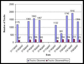
Figure 6-1 summarizes the number of trucks observed each day of the field study. Since the number of hours of data collection varied by day, the number of trucks per hour is also provided to be able to better compare truck volumes by day. The average number of trucks observed traversing the station per day over the two weeks of data collection was about 1,370. This equates to about 179 trucks per hour. Truck volume was greatest on Thursdays and generally higher toward the end of the week. Monday was the slowest day in terms of truck traffic. Data were not collected on weekends. Also, no data collector was present on July 12, and raw truck counts are lower on July 19 due to the station being closed in the late morning and entire afternoon.
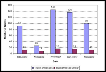
Figure 6-2 shows the total number of trucks and the number of trucks per hour that bypassed the station via NORPASS and hence were captured by the NORPASS system during the second week of the field study. An average of 13.5 trucks per hour bypassed the station via NORPASS during the 37 hours of data collection in the second week. The largest number of bypasses occurred Wednesday through Friday.
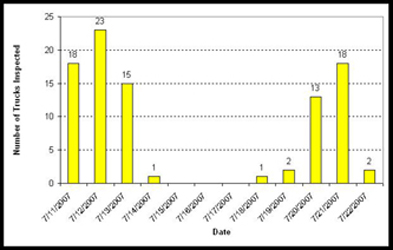
Figure 6-3 illustrates the number of inspections conducted per day at the station. The number of inspections per day varied throughout the course of the two-week study and was driven by the number of inspectors on duty on a given day. During the field study, Laurel County had two new KVE inspectors working for the first time. This was not believed to have a significant effect on the evaluation, nor on the number of inspections achieved per day. The prevailing attitude among inspectors at the time of the study was that the two new inspectors, once trained, might enable the KVE staff at the site to make better use of the ISSES data. The new inspectors were not observed to be using the ISSES equipment any more than the experienced inspectors assigned to the Laurel site. Since no data collector from the evaluation team was present on the weekends, no inspection data was collected on weekends either.
6.4.1 Carrier Demographics
The USDOT number for every truck observed during the field study was cross-referenced with the Motor Carrier Management Information System (MCMIS) Census File to obtain selected demographic information. A large percentage of the truck traffic, 95 percent, was interstate carriers, while the remaining 5 percent operated within the state of Kentucky. The large percentage of interstate carriers is not surprising, given that the station lies along I-75, a main corridor for north/south traffic in that part of the country, and is located just 30 miles north of the Tennessee border.
Table 6-5 shows a breakdown of the trucks' home states. Since license plate information was not captured on all trucks, the home state for each truck is defined as the base state of the truck's carrier as listed in the MCMIS Census File. Roughly 11 percent of the truck traffic was based in Kentucky. Another 25 percent of the trucks had carriers based in three of the states bordering Kentucky (Tennessee, Ohio, and Indiana). A large portion of the truck traffic hailed from the midwest and south with a small percentage based in western states.
| State | Number | Percent |
|---|---|---|
Kentucky |
1,387 |
10.82 |
Tennessee |
1,301 |
10.15 |
Ohio |
1,144 |
8.92 |
Indiana |
773 |
6.03 |
Michigan |
707 |
5.51 |
Arkansas |
685 |
5.34 |
Wisconsin |
593 |
4.62 |
Florida |
564 |
4.40 |
Illinois |
531 |
4.14 |
Ontario, Canada |
477 |
3.72 |
Georgia |
445 |
3.47 |
North Carolina |
409 |
3.19 |
Pennsylvania |
333 |
2.60 |
Nebraska |
288 |
2.25 |
Iowa |
283 |
2.21 |
Alabama |
263 |
2.05 |
Arizona |
243 |
1.89 |
Missouri |
235 |
1.83 |
Texas |
221 |
1.72 |
Minnesota |
194 |
1.51 |
South Carolina |
183 |
1.43 |
Virginia |
175 |
1.36 |
New Jersey |
107 |
0.83 |
All Other States |
1,283 |
10.00 |
TOTAL |
12,824 |
100.00 |
6.4.2 Carrier Electronic Screening
Of the 12,824 observed trucks that traversed the Laurel County inspection station during the times of field study data collection, 639 (or 5 percent) contained a transponder enrolled in NORPASS. Seventy-eight percent of the 639 e-screening participating trucks were allowed to bypass the station while the remaining 22 percent were instructed to pull into the station. This observed pull-in percentage is consistent with what would be expected given the NORPASS pull-in rates provided in Table 6-2. Figure 6-4 illustrates the percentage of trucks that bypassed and pulled into the station each day for the second week of the study. The percentages are fairly consistent across the five days, with a slightly higher pull-in rate on Thursday and Friday.
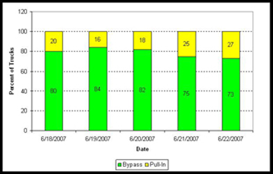
Table 6-6 displays the percentage of trucks that pulled into the station at the direction of NORPASS broken down by the reasons they were pulled in. Over half of the trucks were pulled in because of no weight data available from the mainline WIM. KTC officials commented that weight data may not be available in cases where a truck is straddling the WIM or there is a significant cargo shift while crossing the WIM. This also could indicate a technical problem with the WIMs. Eighteen percent were selected randomly for pull-in, while 13 percent had problems with their credentials or they were identified as a PRISM carrier. About 11 percent were brought in for a weight violation.
| Reason for Pull-In | Percentage of Trucks |
|---|---|
Credentials related or PRISM Carrier |
12.6% |
No weight data |
58.2% |
Random Selection |
17.9% |
Weight Violation |
11.4% |
6.4.3 Carrier Risk
The carriers' ISS scores were used to assess their safety risk. ISS is a decision aid for CMV roadside driver/vehicle safety inspections, which guides safety inspectors in selecting vehicles for inspection. The underlying inspection value is based on data analysis of the motor carrier's safety performance record using information from FMCSA's MCMIS. It is primarily based on SafeStat with an additional carrier-driver-conviction measure. SafeStat ranks all carriers by their safety performance in areas of crash history, inspection history, driver history, and safety management experience (UGPTI 2004). The system provides FMCSA with the capability to continuously quantify and track the safety status of motor carriers, especially unsafe carriers. This allows FMCSA enforcement and education programs to effectively allocate resources to carriers that pose a high risk of involvement in crashes. The ISS provides a three-tiered recommendation, as shown in Table 6-7.
| Recommendation | ISS Inspection Value | Risk Category |
|---|---|---|
Inspect (inspection warranted) |
75 - 100 |
High |
Optional (may be worth a look) |
50-74 |
Medium |
Pass (inspection not warranted) |
1-49 |
Low |
The USDOT numbers for the 12,824 trucks observed at the inspection site were compared with a copy of the SAFER database obtained at the time of the field study to obtain the ISS score for each carrier that could be identified. Trucks were then placed into risk categories based on Table 6-7. Carriers were placed into an "insufficient data" risk category if there was not enough information to generate an ISS score. Carriers with USDOT numbers that could not be found in SAFER were labeled as unknown. The distribution of safety ratings was also generated for all active carriers in the SAFER database at the time of the field study so that a comparison could be made between the relative safety risk for the population of Kentucky traffic around the Laurel County station and the population of CMVs nationally.
Figure 6-5 shows the percent of Kentucky field study truck traffic that fell into each risk category based on each carrier's ISS score, compared with the risk breakdown of all active trucks in SAFER at the time of the field study. A large proportion of the carriers in SAFER, however, about 81 percent, do not have sufficient information to generate an ISS score based on safety information (as opposed to less than 8 percent of the field study truck traffic). This skewed the risk distribution for the national truck population toward the Insufficient Data risk category. To better compare the Kentucky carriers with the national carriers, only carriers with sufficient information from SAFER were used. Also, unknown carriers (ones where USDOT numbers could not be matched to SAFER) were removed from this particular comparison.
About 33 percent of the Kentucky field study truck traffic is considered high-risk based on ISS while 21 percent and 46 percent are considered medium- and low-risk, respectively. The percentage of national high-risk carriers is lower than in Kentucky. As mentioned previously, there were a large number of carriers in SAFER with insufficient information to place them in a risk class—much more so than in the truck traffic for Kentucky. Furthermore, an examination of historical inspection reports from Kentucky has indicated that carriers with insufficient data to generate an ISS score have OOS rates comparable to those trucks in the high-risk category. Consequently, the exclusion of all carriers from SAFER with insufficient data may be artificially lowering the percentage of high-risk carriers from a national perspective. Regardless, the risk distribution of Kentucky truck traffic does not differ dramatically from that of the national risk breakdown. Furthermore, the percentages of trucks by risk are relatively consistent with results obtained from three other field studies conducted in Colorado, New York, and Ohio as part of the separate Evaluation of the National CVISN Deployment Program (not shown here). As a result, it is reasonable to assume that the traffic near the Laurel County station is comparable to the national population of carriers from a risk standpoint.
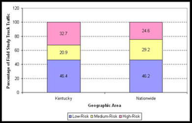
- Kentucky truck traffic based on 11,515 observed trucks during June 11 – June 22, 2007 with sufficient information to calculate ISS score.
- National data based on approximately 219,000 carriers in SAFER Carrier Table with sufficient information to calculate ISS score.
In addition to assessing the safety risk distribution for Kentucky truck traffic versus the national carrier population, risk classification was also used to compare different segments of the Kentucky truck traffic observed during the field study. Table 6-8 examines the risk distribution (based on ISS scores) of Kentucky field study trucks with and without transponders.
| ISS Risk Classification | # of KY Field Study Trucks Screened with Transponder | % | # of KY Field Study Trucks Screened without Transponder | % |
|---|---|---|---|---|
High |
83 |
13.0 |
3,677 |
30.2 |
Medium |
91 |
14.2 |
2,315 |
19.0 |
Low |
459 |
71.9 |
4,890 |
40.1 |
Insufficient Data |
4 |
0.6 |
996 |
8.2 |
Unknown |
2 |
0.3 |
307 |
2.5 |
Total |
639 |
100.0 |
12,185 |
100.0 |
Of all trucks participating in e-screening, about 72 percent are classified as low-risk compared to only 40 percent of non e-screening participating carriers. Thirteen percent of e-screening carriers are in the highest risk class as opposed to more than 30 percent of trucks without transponders. This is not surprising, because carriers with better safety records are more likely to enroll in e-screening than carriers with poorer safety records.
Table 6-9 examines the risk distribution of all e-screening participating carriers who were given a green light to bypass the station as well as those instructed to pull into the station. Based on the objectives of e-screening, one would expect a larger percentage of high-risk trucks to be pulled in versus allowed to bypass. The data support this expectation as the set of bypassed trucks have a lower percentage of high-risk trucks (about 11 percent) compared to the trucks instructed to pull in (about 21 percent). Again this is not surprising given that the rate in which trucks are pulled into stations is higher for those trucks with higher carrier's vehicle and driver OOS rates. Lower risk trucks are pulled in less frequently.
| ISS Risk Classification | # of KY Field Study Trucks that Bypassed Station | % | # of KY Field Study Trucks that Pulled In | % |
|---|---|---|---|---|
High |
53 |
10.6 |
30 |
21.3 |
Medium |
78 |
15.7 |
13 |
9.2 |
Low |
361 |
72.5 |
98 |
69.5a |
Insufficient Data |
4 |
0.8 |
0 |
0.0 |
Unknown |
2 |
0.4 |
0 |
0.0 |
Total |
498 |
100.0 |
141 |
100.0 |
6.5 Inspection Efficiency
For purposes of this evaluation, inspection efficiency is defined by the degree to which inspectors choose high-risk trucks for inspection. A high-risk truck is one where there is a high likelihood that the truck is operating with a serious OOS condition. There are multiple ways to define the risk associated with a truck. Two methods explored in this section are: (1) the carrier's ISS score, a rating system promoted by USDOT; and (2) a carrier's vehicle and driver OOS rates, which are the metrics currently preferred by Kentucky in roadside enforcement.
6.5.1 Risk Categories Using Carrier ISS Score
The data that were needed to assess the efficiency of the current inspection practices included the following:
- ISS Risk classifications for trucks in the population at the inspection site (based on observed truck traffic during field study);
- ISS Risk classifications for trucks that were inspected (based on approximately 2.5 years of state inspections in Kentucky); and
- OOS rates by ISS risk classification, historically, and during the field observational studies.
As discussed in Section 6.4.1, trucks observed at the inspection site were placed into one of five risk categories based on the carrier's ISS score. Using the same methodology, risk classifications based on the ISS score were also obtained for trucks inspected at both the Laurel County north- and southbound stations from January 2005 through mid-September 2007. In order to obtain OOS rates by risk category, the historical inspection records were used to determine whether each inspection over the 32.5 month timeframe resulted in an OOS order being issued. OOS rates were expressed as the number of OOS orders given per 100 inspections for each risk category.
For trucks inspected anywhere in Kentucky from January 2005 through mid-September 2007, the carrier's risk category at the time the inspection took place is not known. The risk category used in the present analysis is based on a copy of SAFER obtained during the field study. The assumption here is that a carrier's current risk rating is the same as when the carrier's vehicle was inspected. A carrier's rating could, of course, have changed over the 2.5-year period. However, based on the availability of SAFER datasets, the rating was assumed to remain constant.
6.5.2 Risk Categories Using Carrier's Vehicle and Driver OOS Rates
Kentucky's use of OOS rates to select vehicles for inspection was described in Section 6.2. For purposes of this discussion, driver OOS rates are multiplied by 3 to make the vehicle and driver OOS rates more comparable numerically. Also, high-risk vehicles are defined as those operated by a carrier with a vehicle or driver OOS rate of at least 25 percent. Medium-risk vehicles are those with a vehicle or driver OOS rate between 10 and 25 percent. Low-risk carriers have OOS rates of at most 10 percent.
OOS rate risk classifications were obtained for the observed truck traffic during the field study as well as vehicles inspected at the north- and southbound Laurel County sites over the previous 2.5 years by cross-referencing each vehicle's USDOT number with the Kentucky Clearinghouse. Then, because there is a wide range of OOS rates for each risk category (e.g., 76 to 99), the average OOS rate for all carriers in each OOS risk category was calculated using historical state inspections. This average number of OOS orders was used in the safety benefits analysis.
6.5.3 Using Carrier ISS Score to Define Truck Risk
Table 6-10 summarizes the inspection efficiency at the Laurel County inspection station in terms of the probability of selecting high-risk trucks. Actual vehicle inspection totals by risk category in the first row are based on more than 17,000 inspections performed at the Laurel County north- and southbound stations between January 1, 2005, and September 13, 2007. Since only 93 trucks were inspected at the northbound ISSES site during the two-week field study,4 the use of the historical inspections provided a more robust risk distribution of inspections. Also for this reason, inspections from the southbound Laurel County station were included. The southbound station is located on the other side of the highway and is similar in layout to the northbound station, with the exceptions that the southbound station does not have an ISSES, and the southbound station has both the low-speed bypass lane and the static scale lane on the east (highway) side of the scale house. The truck traffic vehicle totals in the second row are based on the total number of trucks observed traversing the station during the field study. The vehicles selected for inspection as well as those in the truck traffic population were divided into high-, medium-, and low-risk, insufficient data, and unknown risk based on the ISS scores of the carrier and are shown in columns 2 through 5 of Table 6-10.
For the inspected and truck traffic vehicles, the probability of a truck being high-risk is shown. The probability of a truck being in the high-risk category is calculated as the number of high-risk trucks divided by the total number of trucks. About 29 percent of the truck traffic at Laurel County was considered high-risk, while 34 percent of the vehicles inspected at the Laurel County station were high-risk. The ratio of the proportion of high-risk vehicles inspected to the proportion in the truck traffic population is 1.16 (33.94 percent divided by 29.32 percent). This ratio is statistically significantly greater than 1 (the value expected if there was no difference between random inspections and current practices). Thus, current inspection practices such as inspector judgment, visual observation of vehicles, and use of NORPASS for transpondered vehicles yield slightly more high-risk trucks than if inspectors would simply choose trucks randomly.
| Vehicle Data | Number of Trucks by Risk Classification | Percent of High-Risk Carriers | ||||
|---|---|---|---|---|---|---|
| High | Med/ Low | Insuff. Data | Unknown | Total | ||
Inspected(1) |
5,929 |
10,502 |
987 |
53 |
17,471 |
33.94% |
Truck Traffic(2) |
3,760 |
7,755 |
1,000 |
309 |
12,824 |
29.32% |
Inspected vs. Truck Traffic |
1.16 |
|||||
(2)* Truck Traffic totals based on more than 12,800 trucks observed during two-week field study at Laurel County Station
The analysis comparing OOS rates for different inspection selection strategies requires estimates of OOS rates across risk categories. Table 6-11 shows statewide OOS rates by risk categories, which were calculated using all inspections in Kentucky between January 1, 2005, and September 13, 2007. OOS rates were 7.2 per 100 inspections for low-risk trucks and 17.2 per 100 inspections for high-risk trucks. OOS rates for trucks with insufficient data and for an unknown risk class were higher than those for high-risk trucks. The overall OOS violation rate was 13.6% over the 32.5-month span.
| Risk Class (Based on ISS Score) | Number of Inspections | Number of Inspections with an OOS Violation | OOS Rate (No. per 100 Inspections) |
|---|---|---|---|
High-Risk |
70,803 |
12,183 |
17.2 |
Medium-Risk |
40,818 |
5,597 |
13.7 |
Low-Risk |
80,225 |
5,763 |
7.2 |
Insufficient Data |
26,384 |
5,072 |
19.2 |
Unknown |
4,222 |
1,561 |
37.0 |
Total |
222,452 |
30,176 |
13.6 |
Kentucky's historic OOS rates were found to be significantly below the national average. Nationally, 24 percent of vehicles inspected were put OOS for vehicle violations and 7 percent of drivers inspected were put OOS for driver violations in 2005 (USDOT 2005b). Based on Kentucky inspections performed from January 1, 2005, through September 13, 2007, Kentucky's vehicle and driver OOS rates for 2005 were 9.5 percent and 4.7 percent, respectively. Representatives of the KTC acknowledged that Kentucky's OOS rates are below the national average and that FMCSA and the Commissioner of KVE have identified the raising of OOS rates as a priority. The KTC has been performing a detailed analysis of Kentucky's OOS rates in an attempt to better understand the difference in OOS rates between Kentucky and the rest of the nation. At the time of this evaluation, no results or conclusions from this analysis were available. More discussion on the relatively low Kentucky OOS rates is provided in Section 6.6.
Table 6-12 presents the results of the analysis of OOS rates. The expected number of OOS orders was calculated for two scenarios: if trucks were selected randomly for inspection, and if trucks were selected according to current practices. The expected number of OOS orders per 100 inspections under each of these scenarios was calculated by multiplying the proportion of trucks in each risk category by the OOS rate for that category. That is, the number of OOS orders per 100 inspections was equal to the proportion of those 100 inspections that would be expected to be in the risk category multiplied by the OOS rate for the risk category. For example, the table illustrates that about 29 percent of trucks observed during the field study were classified as high-risk compared to roughly 34 percent of the inspections conducted at the Laurel County station. The state OOS rate for the high-risk category is 17.2. Thus, the expected number of OOS orders per 100 random inspections of high-risk trucks would be 5.04 (29.32*0.172). Using current inspection practices, the expected number of OOS orders per 100 inspections for high-risk trucks is 5.84 (33.94*0.172). Within each inspection selection scenario, the sum of the corresponding numbers over all five risk categories gave the total number of OOS orders expected per 100 inspections.
| ISS Risk Category | Percentage of Commercial Vehicles< | State OOS Rate | No. OOS Orders per 100 Inspections | ||
|---|---|---|---|---|---|
| Random Selection(1) | Inspected(2) | Random Selection | Inspected | ||
High |
29.32 |
33.94 |
17.2 |
5.04 |
5.84 |
Medium |
18.76 |
18.43 |
13.7 |
2.57 |
2.52 |
Low |
41.71 |
41.68 |
7.2 |
3.00 |
3.00 |
Insufficient Data |
7.80 |
5.65 |
19.2 |
1.50 |
1.08 |
Unknown |
2.41 |
0.30 |
37.0 |
0.89 |
0.11 |
Total Expected OOS Orders per 100 Inspections |
13.00 |
12.55 |
|||
(2) Actual selection percentages are based on more than 17,000 inspections performed at the Laurel County northbound and southbound stations between January 1, 2005 and September 13, 2007.
Overall, if trucks were selected for inspection at random, one would expect about 13 OOS orders per 100 inspections. Using the current inspection selection procedure, the number of OOS orders per 100 inspections would be expected to drop 0.45 OOS orders per 100 inspections. Although the number of OOS orders for high-risk trucks increases, the slight overall drop in OOS orders is due mainly to the lower percentage of insufficient data carriers that are inspected compared to the percentage of carriers with insufficient data in the truck traffic population. This is a consequence of Kentucky focusing on OOS rates as a measure to select high-risk trucks—if any historical safety data were used at all—and not using ISS scores to select vehicles for inspection. Moreover, the state OOS rate for insufficient data carriers is quite high at 19.2 OOS orders per 100 inspections. Thus, current inspection selection practices do not yield an improvement in the number of OOS orders over selecting trucks randomly.
Table 6-13 illustrates the impact on the number of OOS orders per 100 inspections where an inspection selection strategy is adopted that incorporates the use of full electronic screening. Under this hypothetical scenario, all CMVs classified as low- and medium-risk enroll in NORPASS, are equipped with transponders, and are allowed to bypass inspection sites. Inspectors then use current practices to select vehicles for inspection from the remaining trucks in the high-risk and insufficient data categories. The second column again shows the risk distribution of trucks that would be expected if trucks were selected randomly for inspection. The third column shows the proportion that would be inspected if all low- and medium-risk trucks were allowed to bypass the site and if the numbers for the remaining risk categories were increased proportionally. For example, the percentage of high-risk trucks expected to be inspected under this strategy would be 74.17 percent {74.17% = 29.32% / [1-(0.1876+0.4171)]}, while no medium- or low-risk trucks would be inspected. As in the preceding table, the expected number of OOS orders per 100 inspections under each of these two scenarios was calculated by multiplying the proportion of trucks in each risk category by the OOS rate for that category. Within each inspection selection scenario, the sum of the corresponding numbers over all five risk categories gave the total number of OOS orders expected per 100 inspections.
| ISS Risk Category | Percentage of Commercial Vehicles | State OOS Rate | No. OOS Orders per 100 Inspections | ||
|---|---|---|---|---|---|
| Random Selection(1) | Full ES(2) | Random Selection | Full ES | ||
High |
29.32 |
74.17 |
17.2 |
5.04 |
12.76 |
Medium |
18.76 |
0.00 |
13.7 |
2.57 |
0.00 |
Low |
41.71 |
0.00 |
7.2 |
3.00 |
0.00 |
Insufficient Data |
7.80 |
19.73 |
19.2 |
1.50 |
3.79 |
Unknown |
2.41 |
6.10 |
37.0 |
0.89 |
2.26 |
Total Expected OOS Orders per 100 Inspections |
13.00 |
18.81 |
|||
(2) Distribution was derived from random selection percentages and the assumption that electronic screening will eliminate low and medium-risk carriers from the selection process (e.g., for high-risk category 74.17% = 29.32% / (1-(0.1876+0.4171))).
Again, if trucks were selected for inspection at random, one would expect about 13 OOS orders per 100 inspections. If electronic screening were implemented to the point that all low- and medium-risk trucks would be allowed to bypass the site, the number of OOS orders per 100 inspections would be expected to rise to about 19. This last scenario represents an increase of OOS orders per 100 inspections of about 45 percent from the scenario where trucks are randomly selected for inspection from the population of traversing trucks. It also represents an increase of OOS orders per 100 inspections of about 50 percent compared to current inspection practices.
6.5.4 Using Carrier OOS Rates to Define Truck Risk
Rather than ISS scores, Kentucky uses a carrier's driver and vehicle OOS rate to determine those trucks that should be selected for inspection at stations where an office support assistant is assigned. Trucks observed during the field test were placed into risk categories based on their vehicle OOS rate or their driver OOS rate (multiplied by three), whichever is higher. Carriers with higher vehicle or driver OOS rates are placed into higher risk categories. In turn, the higher the risk category that a truck belongs to, the higher the probability that the truck would be kicked out for inspection.
The USDOT numbers of all trucks observed during the field study were cross-referenced with a copy of the Kentucky Clearinghouse database near the time of the field study to obtain both the vehicle and driver OOS rate for each carrier. Based on the higher of the vehicle and driver (multiplied by three) OOS rates, carriers were placed into one of seven risk categories.
The first three columns in Table 6-14 show the risk categories as well as the risk distribution for the Kentucky field study truck traffic. Carriers are defined as having insufficient data if no inspection information was available for that carrier in SAFER. Unknown trucks are operated by carriers whose USDOT number could not be found in SAFER. About 63 percent of the truck traffic have carriers in the 0-24 risk class. Five percent of the truck traffic had OOS scores above 50.
To evaluate the inspection selection efficiency associated with the Kentucky inspection selection algorithm, the next set of columns summarizes information used to simulate what would happen if inspectors followed the algorithm explicitly. The percentage of trucks that would be kicked out for inspection based on the distribution of truck traffic observed during the field study is provided as well as the kick-out rates for each risk category. The inspection kick-out rates are defined as the number of trucks that the algorithm identifies for inspection and are the standard rates used by KVE personnel as of June, 2007. These rates could be altered by KVE as needed to change the focus of their inspections. However, for this illustration the standard rates are used. Also, the rates for unknown and insufficient data are set at 1 in 500 trucks, the same as the lowest risk category. The number of observed trucks in each risk category is multiplied by the kick-out rate to identify the number and percentage of observed trucks that would be identified by the algorithm for possible inspection.
| Risk Category (Based on OOS Score) | Truck Traffic | Kicked Out Trucks | |||
|---|---|---|---|---|---|
| # Trucks | Percent | Inspection Kick-out Rate |
# Trucks | Percent | |
100 |
41 |
0.32 |
1/20 |
2 |
1.61 |
76-99 |
155 |
1.21 |
1/5 |
31 |
25.00 |
50-75 |
442 |
3.45 |
1/10 |
44 |
35.48 |
25-49 |
2,808 |
21.89 |
1/100 |
28 |
22.58 |
0-24 |
8,071 |
62.94 |
1/500 |
16 |
12.90 |
Insuff Data |
1,000 |
7.80 |
1/500 |
2 |
1.61 |
Unknown |
307 |
2.39 |
1/500 |
1 |
0.81 |
Total |
12,824 |
100.00 |
124 |
100.00 |
|
Approximately 124 trucks would have been kicked out by the Kentucky OOS rate inspection selection algorithm over the 8.5 days of data collection (or about 14.6 trucks per day). The number of kicked out trucks was arrived at based on the time a researcher was present to capture truck identification information—roughly an 8-hour inspector work day. As designed by the algorithm, the kicked out trucks were spread throughout all risk categories with more emphasis on the higher OOS rate categories. About 25 percent of kicked out trucks had OOS rates in the 76 to 99 range while 35 percent had OOS rates in the 50 to 75 range. Examination of the risk distribution of truck traffic at the station during the field study, as shown in the second and third columns of Table 6-14, shows that the risk distribution of truck traffic is significantly lower—only about 1.5 percent of trucks had an OOS rate in the 76 to 100 range and 3 percent in the 50 to 75 range. Roughly 63 percent of trucks had OOS rates in the 0 to 24 range.
Table 6-15 summarizes the inspection selection efficiency that would be obtained if the algorithm was used explicitly. For both the truck traffic and kicked out vehicles, the probability of a truck being of high risk is shown where high-risk is defined as trucks having an OOS score in the 25 to 100 range. For example, the probability of selecting a high-risk truck if the selection process was purely random is about 27 percent. However, the percent of high-risk trucks kicked out for inspection using the OOS rate algorithm is much higher, at almost 85 percent.
The proportion of high-risk vehicles kicked out for inspection divided by the proportion in the truck traffic population is 3.16. This ratio is also statistically significantly greater than 1. Thus, the inspection selection process where inspectors focused only on trucks that were kicked out for inspection based on the OOS rate algorithm would result in more than three times as many high-risk carriers than would be inspected if the selection were purely random.
| Vehicle Data | Percent of High-risk Carriers (OOS >24) |
|---|---|
Truck Traffic |
26.87% |
Kicked Out Trucks |
84.90% |
Kicked Out vs. Truck Traffic Population |
3.16 |
To further examine the inspection efficiency of the Kentucky inspection selection algorithm, an analysis was performed to compare the number of OOS orders issued under the various scenarios. The analysis comparing OOS rates requires estimates of OOS rates across risk categories. Table 6-16 shows statewide OOS rates by risk categories, which were calculated using all inspections in Kentucky between January 1, 2005, and September 13, 2007. The total number of inspections during this time frame, 222,452, represents all inspections at fixed and mobile sites conducted throughout the state. OOS rates ranged from 7.9 per 100 inspections for trucks with OOS rates between 0 and 24 to 39.6 per 100 inspections for trucks with a 100 percent OOS rate. The overall OOS violation rate was 13.6 percent over the 32.5-month span.
The OOS rate presented in the last column is the main driver for determining the OOS rate risk category (column 1) to which a carrier belongs. Because of this, carriers in riskier categories have higher OOS rates. Because there is a wide range of OOS rates for each risk category, the purpose of Table 6-16 is to get the average OOS rate for all carriers in each OOS risk category. This average OOS rate for each risk category was used in the subsequent analysis of OOS orders per 100 inspections.
Table 6-17 presents the results of the analysis of OOS rates. The expected number of OOS orders was calculated for two scenarios: if trucks were selected randomly for inspection, and if trucks were selected using the Kentucky OOS rate algorithm. The expected number of OOS orders per 100 inspections under each of these scenarios was calculated by multiplying the proportion of trucks in each risk category by the OOS rate for that category. That is, the number of OOS orders per 100 inspections was equal to the proportion of those 100 inspections that would be expected to be in the risk category multiplied by the OOS rate for the risk category. For example, the table illustrates that about 1.21 percent of trucks observed during the field study had an OOS rate in the 76 to 99 range compared to roughly 25 percent of the kicked out vehicles. The state OOS rate for this risk category is 29.9 percent. Thus, the expected number of OOS orders per 100 random inspections of trucks having an OOS rate in the 76 to 99 range would be 0.36 (0.0121*29.9). Using the Kentucky OOS Rate Algorithm, the expected number of OOS orders per 100 inspections is 7.46 (0.2496*29.9). Within each inspection selection scenario, the sum of the corresponding numbers over all seven risk categories provides the total number of OOS orders expected per 100 inspections.
| OOS Rate Risk Category | Number of Inspections | Number of Inspections with an OOS Violation | OOS Rate (No. per 100 Inspections) |
|---|---|---|---|
100 |
2,068 |
818 |
39.6 |
76-99 |
4,726 |
1,413 |
29.9 |
50-75 |
15,890 |
3,786 |
23.8 |
25-49 |
54,464 |
8,484 |
15.6 |
0-24 |
114,756 |
9,052 |
7.9 |
Insuff Data |
26,384 |
5,072 |
19.2 |
Unknown |
4,164 |
1,551 |
37.2 |
Total |
222,452 |
30,176 |
13.6 |
| OOS Rate Risk Category | Percentage of Commercial Vehicles | State OOS Rate | No. OOS Orders per 100 Inspections | ||
|---|---|---|---|---|---|
| Random Selection(1) | Kicked Out(2) | Random (based on population) | Random (based on kick-outs) | ||
100 |
0.32 |
1.61 |
39.6 |
0.13 |
0.64 |
76-99 |
1.21 |
25.00 |
29.9 |
0.36 |
7.48 |
50-75 |
3.45 |
35.48 |
23.8 |
0.82 |
8.44 |
25-49 |
21.89 |
22.58 |
15.6 |
3.41 |
3.52 |
0-24 |
62.94 |
12.90 |
7.9 |
4.97 |
1.02 |
Insufficient Data |
7.80 |
1.61 |
19.2 |
1.50 |
0.31 |
Unknown |
2.39 |
0.81 |
37.2 |
0.89 |
0.30 |
Total Expected OOS Orders per 100 Inspections |
12.08 |
21.71 |
|||
(2) Kick-out rate distribution was derived using the risk distribution of the more than 12,000 vehicles that were observed at the Laurel County northbound inspection site during the field study and the corresponding kick-out rate for each risk category.
Overall, if trucks were selected for inspection at random, one would expect about 12 OOS orders per 100 inspections. Using the Kentucky OOS rate algorithm to select trucks, the number of OOS orders per 100 inspections would be expected to rise to almost 22. This represents an increase of OOS orders per 100 inspections of about 80 percent from the scenario where trucks are randomly selected for inspection from the population of traversing trucks. Moreover, this inspection selection strategy yields 15 percent more OOS orders than the scenario where electronic screening is performed based on ISS scores and allows all low-and medium-risk carriers to bypass. This is to be expected since the Kentucky algorithm focuses solely on OOS rates for screening while ISS scores are comprised of a number of different safety measures.
In summary, the inspection selection efficiency at the Laurel County station is very similar to the efficiency that would be obtained if trucks were selected randomly from the population of traversing trucks. The percent of high-risk trucks selected for inspection under current roadside enforcement measures is slightly higher than the percentage that would be obtained through a purely random selection. However, the number of OOS orders issued under these two scenarios is not significantly different. These results are based on data collected from a site that does not as yet have a fully operational and integrated ISSES system, nor does the system employ a significant amount of inspection selection criteria beyond visual inspection, inspector experience, or inspector judgment.
As Table 6-17 illustrates, inspection efficiency could be significantly improved if the Kentucky OOS rate algorithm were consistently used to identify vehicles for inspection. The use of this algorithm requires two things: 1) every truck that traverses the inspection station needs to be instantly identified (e.g., USDOT number, KYU number, license plate number); and 2) this identifying information needs to be linked to federal or state databases such as the Kentucky Clearinghouse to obtain the necessary historical safety information needed to identify trucks for inspection in real time. A fully operational and integrated ISSES would provide the necessary means for inspectors to use this algorithm to improve inspection selection efficiency. The USDOT and license plate cameras would record the truck identification information while integration with data sources such as SAFER or the Kentucky Clearinghouse would provide inspectors the instantaneous, real-time access to carrier and truck information needed to make better inspection decisions.
6.6 Safety Benefits
Table 6-18 presents a summary of large trucks involved in crashes in 20055 both nationally and within Kentucky.
| Kentucky | Nation | |
|---|---|---|
Large Trucks involved in Crashes |
2,853 |
441,000 |
Fatalities |
124 |
5,212 |
Injuries |
1,858 |
114,000 |
Fatality Analysis Reporting System (FARS), MCMIS.
The most important benefit expected from the deployment of the ISSES and other CVISN technologies, especially electronic screening and safety information exchange, is a reduction in CMV related crashes through improved enforcement of the Federal Motor carrier'safety Regulations (FMCSRs). The principal hypothesis to be tested is that the ISSES and CVISN technologies will help enforcement staff focus inspection resources on high risk carriers. This will result in more OOS orders for the same number of inspections—thereby removing from service additional trucks and drivers that would have caused crashes because of vehicle defects and driver violations of safety regulations.
6.6.1 Technical Approach
The following sections describe (1) the sources of data obtained from the literature and the field study conducted at the Laurel County station used to estimate the impacts of ISSES and CVISN on roadside safety enforcement, (2) the crash avoidance model used to estimate safety benefits, and (3) various roadside enforcement (RE) scenarios used to illustrate the safety benefits.
Data Sources
Table 6-19 lists some key safety statistics obtained from the published literature. Most of these data are used in the crash avoidance analysis; others are provided for reference. According to FMCSA, 8.5 million large trucks (>10,000 pounds gross vehicle weight) in 2005 traveled approximately 233 billion miles in the U.S. Also in 2005, the last year for which complete statistics are available, 441,000 trucks were involved in crashes, resulting in approximately 114,000 injuries and 5,212 deaths. The corresponding rates per vehicle mile traveled are derived from these values. Other relevant statistics provided in Table 6-19 include the number of national and Kentucky CMV inspections performed in 2005 and the actual percentages of OOS orders issued. In 2003, FMCSA sponsored the National Truck Fleet Safety Survey (TFSS), in which approximately 2,800 trucks were selected at random for inspection in order to estimate the percentages of trucks and drivers that operate with OOS conditions (i.e., violation rates). These estimates differ from the actual OOS rates because inspectors choose vehicles for inspection based on vehicle appearance and apply their knowledge and experience. The estimated OOS rates reported by the TFSS were 28 percent for vehicles and 5 percent for drivers (FMCSA 2006b).
In order to determine the impact of removing OOS violators from the roadway on the number of crashes, it is necessary to estimate certain probabilities associated with crash causation. One important component to the statistical crash reduction model is being able to estimate the relative risk of driver and vehicle OOS violations in truck crashes. Specifically, we would like to know the probability that an OOS condition exists on a truck given a crash has occurred involving that truck. Before the FMCSA-sponsored Large Truck Crash Causation Study (LTCCS), there were not reliable estimates of this probability for either vehicle or driver OOS violations as there had not been sufficient data to support calculation of reliable estimates. By focusing on the pre-crash condition of the truck, the LTCCS provides the right type of data for this analysis. The LTCCS data was used to calculate various probabilities that were used as inputs to the crash avoidance model (USDOT 2006a). These data are discussed more fully in the next section along with the explanation of the crash avoidance model.
| Statistic Description | Value | Source 1 |
|---|---|---|
Number of large trucks |
8.5 million |
Large Truck Crash Facts 2005 (USDOT 2007b) |
Large truck annual vehicle miles traveled (VMT) |
233 billion |
Large Truck Crash Facts 2005 (USDOT 2007b) |
Large trucks involved in crashes (2005) Injuries from large truck crashes (2005) Fatalities from large truck crashes (2005) |
441,000 114,000 5,212 |
Large Truck Crash Facts 2005 (USDOT 2007b) |
Large trucks involved in property damage-only crashes Large trucks involved in injury-only crashes Large trucks involved in fatal crashes |
354,000 82,000 4,932 |
Large Truck Crash Facts 2005 (USDOT 2007b) |
Large truck crash rate (truck crashes/100 million VMT) = 441,000 truck crashes/233 billion VMT |
189.3 |
Derived |
Commercial vehicle (non-bus) vehicle inspections performed (2005) Commercial vehicle (non-bus) driver inspections (2005) Total CV (non-bus) inspections (driver or vehicle) (2005) Kentucky annual commercial vehicle (non-bus) vehicle inspections performed (2005) Kentucky annual commercial vehicle (non-bus) driver inspections performed (2005) Kentucky annual commercial vehicle (non-bus) (driver or vehicle) inspections performed (2005) |
1,949,375 2,669,679 2,708,856 44,142 86,028 86,077 |
Annual Summary of Roadside Inspections - NAFTA Safety Stats (A&I website) Kentucky Historical Inspection Data |
Percent of vehicles placed OOS (2005) Percent of drivers placed OOS (2005) Kentucky percent of vehicles placed OOS (2005-Sept 2007) Kentucky percent of drivers placed OOS (2005 – Sept 2007) Kentucky percent of vehicles or drivers placed OOS (2005 – Sept 2007) |
24.0% 7.0% 9.5% 4.7% 13.6% |
Annual Summary of Roadside Inspections - NAFTA Safety Stats (A&I website) Kentucky Inspection Data (2005 – Sept 2007) |
Percent of VMT with vehicle OOS conditions (2003) Percent of VMT with driver OOS conditions (2003) Percent of inspections that found at least one OOS vehicle violation given a OOS driver violation was found Percent of VMT with brake-related OOS conditions |
28% 5% 49% 14% |
2003 National Truck Fleet Safety Survey (TFSS) (USDOT 2006b) 1996 National Survey (Star 1997) |
Percent of large CMV crashes with vehicle OOS condition present |
32.4% |
Derived from LTCCS |
Percent of large CMV crashes with driver OOS condition present |
17.2% |
Derived from LTCCS |
While these data provide much of the necessary information needed to estimate safety benefits, additional data from the inspection efficiency field study conducted at the Laurel County inspection station were needed to supplement the data in Table 6-19. Specifically, information on the rate at which OOS orders were issued at the Laurel County station were used as well as the calculated increase in the OOS order rate under different roadside enforcement scenarios.
Crash Avoidance Model
Ultimately, safety benefits will be realized only to the extent that targeted inspections and improved compliance translate into reductions in numbers of crashes. The premise of targeted inspections is that, for the same number of inspections performed, additional drivers and vehicles operating with OOS conditions will be removed from the roadway. Furthermore, all of the conditions leading to the OOS order will be fixed and "stay fixed" for a period of time after the inspection. Therefore, crashes that would have occurred during this period are prevented because the OOS conditions that would have caused the crashes were eliminated. The safety benefit of ISSES and CVISN technologies is determined by comparing the number of crashes avoided under a baseline scenario (i.e., with pre-ISSES or CVISN roadside enforcement strategies and technology) with the number of crashes avoided under a number of deployment scenarios involving the ISSES and CVISN. It is assumed under each scenario that the corresponding number of injuries and fatalities avoided are proportional to the number of crashes avoided.
The basic principle of the crash avoidance model, as well as certain assumptions about how roadside enforcement affects crash rates, were motivated by research on the Safe-Miles model developed for FMCSA to estimate the benefits of MCSAP, the Motor carrier'safety Assistance Program (VNTSC 1999). Although the model used in the Kentucky safety benefits analysis is different from the one used in Safe-Miles, certain model parameters such as the number of "safe miles" a truck travels following an OOS order, are used in this analysis. The approach to safety benefits estimation in the Kentucky evaluation was adapted from the approach documented in Chapter 5 of the CVISN Model Deployment Initiative (MDI) Evaluation (USDOT 2002).
In simplest terms, the number of crashes avoided can be written as
![]() (1)
(1)
where
- P(V|inspection) is the probability that a truck has an OOS violation given that it was inspected
- P(C|V) is the probability of a crash given that a vehicle has an OOS violation
-
 is the probability of a crash given that a vehicle does not have an OOS violation.
While the number of inspections and the probability of a violation given an inspection are easily obtained, the probability of a crash given that a vehicle has an OOS condition as well as the probability of a crash given that a vehicle does not have an OOS condition are more complicated. Using Bayes Theorem, we rewrite P(C|V) and ![]() as
as
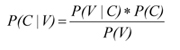 (2)
(2)
![]() (3)
(3)
where
- P(V|C) is the probability that a vehicle has an OOS violation given it is in a crash
- P(C) is the probability of a crash
- P(V) is the probability that a vehicle has an OOS condition
 is the probability that a vehicle does not have an OOS violation given it is in a crash
 is the probability that a vehicle does not have an OOS condition.
Substituting the new expressions for P(C|V) and ![]() presented in Equations (2) and (3) into Equation (1) and performing some algebraic manipulation yields the following model for crashes avoided:
presented in Equations (2) and (3) into Equation (1) and performing some algebraic manipulation yields the following model for crashes avoided:
![]() (4)
(4)
In this analysis, we are only concerned with crashes that are avoided because they would have been caused by a vehicle defect or driver violation that resulted in an OOS order. Also, it is generally assumed that the probability of a crash is proportional to the number of vehicle miles traveled (VMT). Therefore, the probability of a crash (among vehicles that would have been operating with defects or driver violations) is estimated by the national crash rate for large trucks (denoted by λ) multiplied by the number of safe miles (SM) traveled as a result of "fixing" an OOS condition. This is the approach used in the Safe-Miles program. The values of SM used in the Safe-Miles program are 15,000 miles for vehicle OOS orders and 10,000 miles for driver OOS orders.
Thus, the final model for crashes avoided is the following:
![]() (5)
(5)
Equation (5) is used to estimate the safety benefits associated with various ISSES and CVISN deployment scenarios presented in the next section. The national crash rate for trucks, λ, is 441,000 truck crashes divided by 233 billion VMT, or 1.89 crashes per million miles traveled.
Additional data needed for this model include P(V|inspection), the probability of an OOS violation given the truck was inspected, P(V), the probability that a vehicle has an OOS violation, and P(V|C), the probability that a vehicle has an OOS violation given it is in a crash. These values depend on the particular roadside deployment scenario or enforcement strategy under consideration. The LTCCS was used to estimate P(V|C) for various OOS violations and groups of violations. For example, given a crash, the probability of a specific OOS violation (such as brakes) or a group of violations (e.g., vehicle or driver) present on the truck was estimated from the LTCCS data.
6.6.2 Deployment Scenarios
Truck traffic at most inspection sites is very heavy, and inspectors cannot inspect every CMV that passes by. Thus, there needs to be a sound methodology for narrowing down the pool of trucks from which inspectors have to choose. Seven overall scenarios are presented in this section, a few of which have been divided into sub-scenarios. The seven deployment scenarios present different methods for selecting vehicles for inspection with the goal being to select trucks that yield the most OOS orders. Using the crash avoidance model given in Equation (5), these scenarios illustrate the estimated safety benefits of the ISSES and other CVISN technologies.
In the CMV law enforcement community, the term "electronic screening" signifies a transponder-based mainline preclearance system, such as NORPASS, HELP/PrePass, Oregon Green Light, or equivalent. Such systems provide roadside enforcement personnel the ability to detect and identify and (optionally) weigh CMVs at mainline speeds. For purposes of this report, Scenarios RE-3 through RE-6 expand the definition of "electronic screening" to include other means of achieving a similar goal, namely to use computers and telecommunication technology to identify and prescreen vehicles in real time. In Scenarios RE-3 through RE-6, ISSES or an equivalent system is used for identifying trucks moving slowly through a weigh station. The basic function is the same as transponder-based preclearance, the only difference being the truck's speed at the point of decision (red light, pull-in, green-light, bypass). In these four scenarios, it is assumed that some trucks carry transponder tags and some do not. Furthermore, it is assumed that all trucks approaching the station are subject to electronic or computer-based, real-time prescreening—at high or low speeds—as an aid to the inspector's decision process. These four scenarios also diverge from the usual definition of "electronic screening" in that, for purposes of modeling and analysis, they introduce screening decision criteria that are different from the criteria believed to be used in the prevailing mainline e-screening programs or partnerships (NORPASS, PrePass, and Oregon Green Light).
Table 6-20 provides a high-level summary of the seven scenarios presented in this section. A more thorough description of each scenario follows the table.
| Scenario Number | Screening Criteria Used in Scenario | ||||||
|---|---|---|---|---|---|---|---|
| Random Only | Inspector Experience and Judgment | Electronic Screening with Snapshots | KY OOS Rate Algorithm | Vehicle and Driver OOS Rates Using Threshold | Brake and Driver OOS Rates | Infrared Images and Driver OOS Rate | |
RE-0 |
X |
||||||
RE-1 |
X |
||||||
RE-2 |
X |
X |
|||||
RE-3 |
X |
X |
X |
||||
RE-4 |
X |
X |
X |
||||
RE-5 |
X |
X |
X |
||||
RE-6 |
X |
X |
X |
||||
RE-0: Random Selection. Enforcement officers (inspectors) select CMVs for inspection in a random manner without using personal experience, judgment, or any ISSES or CVISN technologies. This is not one of the roadside enforcement strategies being considered, nor is it a realistic strategy to employ. However, the calculation of safety benefits under this scenario is useful for determining the contribution of the inspectors' knowledge and experience during the vehicle selection process.
RE-1: Baseline—Pre-ISSES/CVISN. Inspectors select CMVs for inspection using personal experience and judgment, but without the aid of ISSES or most CVISN technologies. Electronic screening is assumed to be used at its current level as of June 2007. This baseline scenario is analyzed twice. First, safety benefits are calculated based on Kentucky vehicle and driver OOS rates, which are significantly lower than the national average. Then, the analysis is performed assuming that Kentucky's vehicle and driver OOS rates were on par with national estimates—referred to as RE-1a.
RE-2: Mainline Electronic Screening based on ISS Score. State deploys electronic screening with safety snapshots at all major inspection sites. Motor carriers that are classified as low- and medium-risk based on ISS scores (comprising approximately 60 percent of trucks on the road) enroll in the electronic screening program, are equipped with transponders, and are allowed to bypass inspection sites. Inspectors use current practices to select vehicles for inspections from the remaining 40 percent of trucks in the high-risk and insufficient data categories.
RE-3: Electronic Screening based on Kentucky OOS Rate Inspection Selection Algorithm. State utilizes Kentucky OOS rate inspection selection algorithm at all inspection sites that utilize electronic screening. Every vehicle that enters the inspection station is identified accurately by the ISSES' ALPR and USDOT readers. Safety information for each carrier is obtained from the Kentucky Clearinghouse. Based on the safety information, the algorithm identifies trucks for inspection as described in Section 6.2. Inspectors select vehicles for inspection from this pool of identified trucks, while non-identified trucks continue to the mainline. Trucks with transponders are subject to the same algorithm already built into NORPASS.
RE-4: Electronic Screening based on high vehicle and/or driver OOS rates. State utilizes the ISSES and/or electronic screening at all major inspection sites. This scenario is similar to RE-3 in that each truck is screened via the ISSES based on the vehicle and driver OOS rate of the carrier. However, RE-4 differs in that a threshold OOS rate is established for both vehicles and drivers such that all trucks with OOS rates exceeding the corresponding thresholds are brought into the inspection station for inspection, while all others are allowed to bypass inspection sites. The threshold rates are chosen such that only trucks with the highest OOS rates are candidates for inspection. The threshold values can vary depending on both the truck traffic and the rate at which inspections can be performed at the site. As part of RE-4, three specific threshold values are considered.
RE-5: Electronic screening based on high driver OOS or brake violation rates. State utilizes the ISSES and/or electronic screening at all major inspection sites. Each truck is screened via the ISSES based on its OOS or violation rate for violations that have a high relative risk for crash. In this scenario, vehicles are screened based on their brake violation and overall driver OOS rates as they appear in SAFER. A distinction is made here between violation and OOS rates. SAFER contains a violation rate for brakes but not a brake OOS rate. Thus, violation rates are used as a safety index for brake issues, while the driver OOS rate is used to screen for driver issues. Both brakes and driver OOS violations have been found to have a high relative risk for crashes. This scenario differs from RE-4 in that vehicles are screened on their brake violation rate as opposed to their overall vehicle violation rate in an attempt to catch those vehicles that have a violation that has a higher relative risk for crash. Similar to RE-4, all trucks with violation rates exceeding the threshold are candidates for inspection, while all others are allowed to bypass inspection sites. Moreover, the threshold rates are chosen such that only trucks with the highest rates are selected for inspection and the thresholds can vary depending on the amount of inspection personnel available at a given station. As part of RE-5, three specific threshold values are considered.
RE-6: Electronic screening based on infrared screening and high driver OOS violation rate. State utilizes the ISSES at all major inspection sites. Each truck is screened via two criteria: the thermal (IR) imaging system on the ISSES and the driver OOS rate of the carrier. In this scenario, vehicles are screened based on the presence of a brake violation through the IR image produced by the ISSES and the driver OOS rate as it appears in SAFER. This scenario is similar to RE-5 in that both brake and driver OOS violations are used as screening criteria. RE-6 differs from RE-5 in that vehicles are screened for brake violations via IR imaging as opposed to brake violation rates obtained from SAFER. All trucks with a potential brake violation as detected from the IR image or trucks with driver OOS rates exceeding various thresholds are candidates for inspection, while all others are allowed to bypass inspection sites.
RE-0 is the most basic selection process of selecting vehicles randomly and is presented mainly to assess the contribution of the inspectors' knowledge and experience during the vehicle selection process, which is represented in the baseline scenario RE-1. The remaining five scenarios all make use of progressively more involved selection criteria. Electronic screening is employed in RE-2 to eliminate all low- and medium-risk carriers from selection consideration. Although this scenario helps improve inspection selection efficiency by allowing inspectors to focus only on high-risk vehicles or those with insufficient data, there are still too many vehicles remaining in these categories for roadside enforcement officials to inspect them all. As a result, scenarios RE-3 through RE-6 provide various methods to further narrow down the number of vehicles that inspectors have to choose from. RE-3 is based on the Kentucky OOS rate inspection selection algorithm, which selects vehicles for inspection at different rates depending on their OOS rates. RE-4 and RE-5 take a slightly different approach in selecting only those vehicles with the highest probability of having particular kinds of OOS violations as measured by some safety index. RE-6 examines the benefits when IR imaging is used to screen for brake violations.
The calculation of safety benefits for scenarios RE-0 through RE-3 are presented in Section 6.6.2. They are straightforward, based on Equation (5), specific inputs contained in Table 6-19, as well as results from the inspection efficiency analysis of the Laurel County site. Scenarios RE-4, RE-5, and RE-6 are more complicated and hence more information is provided in this section in advance of the results presentation in Section 6.6.2.
RE-4 and RE-5: Methodology for Selecting Vehicles for Inspection Based on Safety Index
The inspection selection strategy described in this section is based on the notion of selecting trucks for inspection based on the value of some safety index associated with the carrier. Any truck with a safety index above a given threshold would be pulled in for inspection while all other trucks would be allowed to bypass the station. The two main issues considered in this section are: 1) Determining the most appropriate safety index; and 2) Determining the threshold value for this index that should be used to decide which vehicles to inspect.
Choice of Safety Index. From an inspection efficiency standpoint, the best choice for a safety index is one that correlates well with the probability of finding an OOS violation on a vehicle chosen for inspection. Further, from a crash prevention standpoint, the OOS violations found should be for violations that pose a high relative risk for crashes. Both viewpoints were used in choosing safety indices. The first set of indices considered in this analysis was the carrier's vehicle and driver OOS rate. Results from the inspection efficiency analysis in Section 6.5 suggest that screening vehicles using carrier OOS rates as opposed to ISS may provide a larger percentage of trucks being placed OOS. As a result, scenario RE-4 focuses on using the carrier's driver and vehicle OOS rate to select vehicles for inspection.
Finding OOS violations during an inspection is crucial to keeping unsafe trucks off the road so that crashes can be prevented. Moreover, a larger number of crashes could be avoided by finding those OOS violations that have a higher relative crash risk. While taking trucks OOS for violations that do not pose a high crash risk serves a benefit, more benefits from a crash reduction and life saving perspective can be realized by focusing on violations related to crash risk. Data from the LTCCS were used to identify those OOS violations that present a high relative crash risk. Every truck involved in a crash within the LTCCS was subject to a full Level I inspection as part of the investigation of each crash. For every truck in the LTCCS that was assigned the critical reason for the crash, inspection reports contained in the LTCCS data were analyzed to record the presence of each type of OOS violation. From this information, the probability of a specific type of OOS violation being present on a truck given that the truck crashed could be calculated by dividing the number of trucks having the violation present by the total number of trucks in a crash. Survey weights associated with the LTCCS were used in these calculations to ensure nationally representative probability estimates.
It is also important to identify OOS violations that occur frequently in the population. A violation that has a high relative risk for crash but that does not appear all that often is not of much use to inspectors because trucks with that violation are too difficult to find. Historical Kentucky inspection data were analyzed to identify the most common OOS violations. For each inspection record, the presence of specific OOS violations was recorded. The probability of a truck having each specific OOS violation was calculated by dividing the number of inspections where the OOS violation was present divided by the total number of inspections.
Table 6-21 presents the probability calculations for both the crash data and the historical Kentucky inspection data for vehicle and driver OOS violations overall as well as six specific types of OOS violations. These six violations were chosen as they were the most frequently occurring violations in both the LTCCS crash data as well as the historical state inspections. The second column presents the probability that a truck has a specific violation given the truck was in a crash. The third column contains the probability that a truck has a specific violation in the population based on the Kentucky historical inspection reports. The assumption here is that past inspections have been random. Now, past inspections are not truly random. However, inspection reports provide the best means of knowing the incidence of OOS violations in the population. Moreover, Table 6-12 showed that the number of OOS orders issued under current Kentucky inspection selection practices was essentially the same if trucks were selected randomly. Thus, the assumption is appropriate for this analysis.
| OOS Violation Categories | Probability of Violation Occurring | |
|---|---|---|
| In a Crash (LTCCS) | In KY (Past Inspection Data) | |
All Vehicle |
32.4% |
9.5% |
Brake Violation |
21.7% |
4.4% |
Lighting |
3.6% |
2.3% |
Tires |
2.9% |
1.5% |
Load Securement |
4.0% |
1.5% |
All Driver |
17.2% |
4.7% |
Log Book |
12.3% |
2.3% |
Hours of Service |
1.6% |
1.3% |
All Violations |
38.72% |
13.6% |
An examination of vehicle violations shows that roughly 22 percent of trucks involved in crashes have a brake violation as compared to only 4 percent in the Kentucky truck population. Lighting, tires, and load securement all occur slightly more frequently in crashes than in the general Kentucky truck traffic population. However, the differences are not as large as brake violations. Driver OOS violations in general had a high relative risk for crash. About 17 percent of trucks involved in crashes have some sort of driver OOS violation as compared to about 5 percent in the Kentucky truck population. Also, analysis of crash data from the LTCCS found that driver related factors were important reasons leading to causes of crashes in a large majority of the cases (USDOT 2006a). As a result, vehicles are selected for inspection in scenario RE-5 based on their likelihood of having a brake violation or general driver OOS violation. Although violations involving the log book have the highest relative risk among driver OOS violations, it was decided to use the more general driver OOS violation rate as opposed to the log book violation rate as an index since the relative crash risks for both measures were similar and since this would better reflect the LTCCS findings regarding general driver-related factors and crash risk. The carrier's driver OOS rates were obtained from the Kentucky Clearinghouse.
The SAFER carrier table does not include a brake OOS rate for each carrier. Rather, a brake violation rate can be calculated from information contained in the table. The brake violation rate is defined as the number of brake violations in the past 30 months divided by the number of vehicle inspections in the past 30 months. Not all brake violations result in an OOS order. Thus, the brake violation rate for each carrier is associated with a probability of a brake OOS rate in the next section. In summary, the brake violation rate and driver OOS violation rate are used as indices in selecting vehicles for inspection in RE-5. The driver OOS violation rate is also used as an index in scenario RE-6, described in greater detail later in this section.
Choice of Index Threshold for Pulling Vehicles in for Inspection. For each safety index used in scenarios RE-4 and RE-5, the next step was to determine a threshold by which any vehicle with a safety index at or above the threshold are brought in for inspection while all vehicles with a safety index below the threshold are allowed to continue on the mainline. The value of the threshold can neither be so high that very few trucks on the road are brought in for inspection nor can it be too low, which would result in more trucks being flagged for inspection than roadside enforcement resources can handle. Moreover, the appropriate value for the index threshold should be dependent on the number of inspectors available at a given inspection site. Consequently, scenarios RE-4 and RE-5 consider three different threshold values for each index, corresponding to the number of trucks that an inspection station could realistically inspect in a given day given its roadside enforcement resources.
Historical Kentucky state inspections were used to determine the specific threshold values for a given index. The various indices (driver OOS rate, vehicle OOS rate, and brake violation rate) for each truck inspected from January 2005 through September 2007 were recorded. For each index, the values of the index were sorted from low to high and the resulting distribution of values was examined so that the 95th, 90th, and 75th percentiles of the distribution were obtained. The 95th percentile of the index distribution is the value where 5% of the trucks meet or exceed that value of the threshold. Since the index values are sorted from low to high, this index value represents the cutoff point for the 5% of trucks with the highest index value. For example, an inspection station with truck traffic of 2,000 trucks per day during normal inspection hours would expect to have about 100 trucks available for inspection if the 95th percentile of the index distribution was used. Using the 90th percentile would result in about 200 trucks available for inspection.
To use Equation (5) to estimate the number of crashes that would be prevented under these scenarios, it is essential to know the probability of a violation given that an inspection occurred for vehicles at or above the index threshold, [i.e., P(V|inspection)]. In order to obtain this probability, it is necessary to understand the relationship between the safety index of the truck and the presence of the specific OOS violation on the truck given an inspection. Each safety index relates to a specific type of OOS order. For instance, a carrier's brake violation rate should be a good predictor that a truck belonging to that carrier has an OOS brake violation. Similarly a carrier's vehicle and driver OOS rate was used to predict the presence of a vehicle or driver OOS violation, respectively.
To gain a better understanding of the relationship between each index and its corresponding OOS violation, a probit regression model was used to model the probability of an inspection having a specific OOS violation against the safety index. Probit analysis is a standard statistical approach to modeling a probability as a function of some continuous explanatory variable. The probit model has the form:
![]() (6)
(6)
where
i = 1, 2, 3, ... corresponding to the total number of distinct values of the index
ρi is the ratio of the number of historical Kentucky inspections that resulted in a specific OOS violation to the number of inspections within each index value i
θ-1 is the inverse of the standard Gaussian distribution function
β0 is the intercept parameter of the probit regression line
β1 is the slope parameter of the probit regression line
xi is the safety index.
Figure 6-6 shows the general form of a probit regression relationship. Given a threshold value xi, the corresponding probability of an OOS violation at that threshold value can be calculated from the probit regression model.
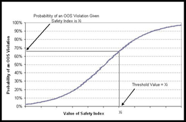
Historical Kentucky inspection data was modeled separately for each of the three indices using the probit model in Equation (6). The probit model for each index was then used to estimate the probability of a corresponding OOS violation given an inspection for each of the three threshold safety index values corresponding to the top 5 percent, 10 percent, or 25 percent of the distribution of the safety index. These probabilities were then used in Equation (5) to capture safety benefits for scenarios RE-4 and RE-5.
RE-6: Methodology for Selecting Vehicles based on Infrared Imaging
Roadside scenario RE-6 is similar to RE-5 in that it focuses on identifying vehicles that have brake and/or driver OOS violations (violations with high relative crash risk). As in RE-5, the driver OOS rate associated with the truck's carrier is used to identify those trucks with a high probability of a driver OOS violation. Threshold values for the driver OOS rate are again used to select an appropriate number of vehicles to bring into the station for inspection. Where RE-6 differs from RE-5 is the manner in which trucks are selected for inspection based on their chances of having a brake violation. Brake problems are difficult to detect with the human eye alone. As a result, alternative techniques need to be adopted to identify trucks with faulty or inoperative brakes. Scenario RE-5 utilizes historical brake safety information on each carrier to identify trucks that were the most likely to have brake problems. There are limitations to this approach. For example, the presence of a high carrier brake violation rate does not guarantee that the specific truck operated by that carrier and now entering the station has a brake violation, just that this truck is more likely to have such a condition, based on the carrier's history.
Thermal (IR) imaging systems provide inspectors with a tool to more accurately identify trucks with brake violations. This coupled with the fact that there is a high relative risk of a crash associated with brake violations, makes the prescreening of vehicles using IR technology a powerful tool that may provide significant benefits in crash reduction. Unfortunately, because of the lack of IR video imaging data from the field study at Laurel County, the benefit of the ISSES thermal imaging system in terms of inspection efficiency and safety benefits cannot be fully assessed for this particular site. However, prior research was conducted in 2000 for FMCSA on evaluating a similar, portable IR imaging and video package, IRISystem (USDOT 2000). Results from the 2000 study are used to estimate the number of crashes, injuries, and fatalities that could be avoided if IR technology were used to screen vehicles.
The objective of the FMCSA 2000 study was to evaluate the effectiveness of the IRISystem for use as a screening tool on CMVs for detecting bad brakes and unsafe vehicles due to braking. A high-level summary of the research and findings, including the increase in OOS rates due to screening vehicles with IR technology, is presented in Appendix D to provide an understanding of the quantifiable benefits that can be realized through use of this technology. However, the key result from this analysis that pertains to scenario RE-6 is that the percentage of vehicles placed OOS due to brake violations after IRISystem screening was 47.2%. This figure is used as an estimate for the probability of a brake violation given that an inspection occurred, [P(V|Inspection)], in Equation (5).
Although they are manufactured by the same company, the IRISystem and ISSES are two different systems. Furthermore, inspection practices and OOS rates vary across states with Kentucky's OOS rate being much lower as described earlier. As such, the estimates of the number of crashes, injuries, and fatalities generated from this exercise provide a general idea of the safety benefits that could be realized using IR technology to screen trucks for brake and tire-related violations and not necessarily the ISSES itself.
6.6.3 Results
In this section the calculations of the numbers of truck crashes, injuries, and fatalities avoided under each of the roadside enforcement scenarios described in Section 6.6.1 are presented. These calculations, based on Equation (5), utilize inputs contained in Table 6-19 as well as specific assumptions defined by the scenarios. Results from special studies are presented as needed to justify some of the parameter estimates used in these models. The safety benefits are expressed in terms of avoided (reduced numbers of) crashes, injuries, and fatalities per year per state, for a state similar to Kentucky in terms of the numbers of commercial vehicle inspections performed per year.
Scenario RE-0: Random Selection
In 2005, the most recent year for which complete data across all sources are available, Kentucky conducted 44,142 vehicle inspections and 86,028 driver inspections. Under random inspections, the proportions of inspected vehicles and drivers that are given OOS orders are equal to corresponding Federal Motor carrier safety Regulation (FMCSR) violation rates. Thus, by applying the results from the National Truck Fleet Safety Survey, 28 percent of the 44,142 vehicle inspections would result in vehicle OOS orders (USDOT 2006b). From Equation (5), the number of crashes that are avoided due to vehicle OOS orders when random inspections are performed is equal to
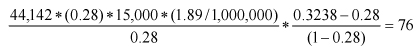 (7)
(7)
Similarly, 5 percent of the 86,028 driver inspections would have resulted in driver OOS order leading to
![]() (8)
(8)
crashes avoided. Note that these two numbers cannot be added to get the total number of crashes avoided because there is some overlap in vehicle and driver OOS orders. To get an estimate of the total number of crashes avoided, the TFSS found that 49 percent of the inspections that found at least one driver OOS violation also found at least one vehicle OOS violation (FMCSA 2006b). Because the impact of vehicle OOS orders is greater than the impact of driver OOS orders, the number of crashes avoided combined over vehicle and driver OOS orders can be determined by adding (a) the number of crashes avoided due to vehicle OOS orders and (b) 51 percent of the crashes avoided due to driver OOS orders. Thus, the total number of crashes avoided would be 76 + (0.51*209) = 183.
Using the injury and fatality data in Table 6-19, there are on average 5,212/441,000 = 0.012 fatalities per crash and 114,000/441,000 = 0.259 injuries per crash. Therefore, if 183 crashes were avoided, it would be expected that 183*0.259 = 47 injuries would be avoided and 183*0.012 = 2 fatalities would be avoided. This relationship between the numbers of crashes, injuries, and fatalities is assumed to hold for all scenarios.
Scenario RE-1: Baseline—Pre-ISSES/CVISN Using Kentucky OOS Rates
The calculation of crashes avoided in the baseline scenario is very similar to the calculation with random selection of vehicles, except instead of applying the results from the TFSS, the actual numbers of OOS orders for vehicles and drivers in Kentucky are used. From January 2005 through mid-September, 2007, 9.5 percent of the vehicle inspections in Kentucky resulted in a vehicle OOS order, and 4.7 percent of the driver inspections in Kentucky resulted in a driver OOS order. In this scenario (and all that follow), the probability of a vehicle and driver OOS violation in a crash as well as in the general population are based on national estimates. This is because: (1) crash probabilities were not available on a state basis from the LTCCS; and (2) reliable estimates of the probability of a violation in the truck population were not possible from Kentucky data due to their significantly lower OOS rates.
Following the approach used with random selection, 9.5 percent of the 44,142 inspections would result in vehicle OOS orders. From Equation (5), the predicted number of crashes avoided due to vehicle OOS orders is equal to
![]() (9)
(9)
Similarly, 4.7 percent of 86,028 driver inspections would result in a driver OOS order leading to
![]() (10)
(10)
crashes avoided.
Applying the 51 percent adjustment factor used under random selection, the estimated number of crashes avoided is 26 + 0.51*197 = 126. The corresponding numbers of injuries and fatalities avoided are 33 and 2, respectively.
Note that the number of crashes avoided due to OOS orders under this scenario is less than the number avoided under the random selection scenario (183 versus 126). This is because the Kentucky vehicle OOS rate used in the calculation (9.5 percent) is significantly lower than the violation rate under the random selection scenario (28 percent) estimated in the TFSS. Overall, Figure 6-7 illustrates that Kentucky's vehicle and driver OOS rates are both lower than their respective national averages as well as being lower than the rates for each of the three states where similar field studies were conducted as part of the National Evaluation of the CVISN Deployment Program. Although there are differences in both vehicle and driver OOS rates, the difference in vehicle OOS rates is more pronounced. The Kentucky driver OOS rate of 4.7 percent is only slightly lower than both the 5 percent rate from the TFSS and the 7 percent rate estimated from the 2005 NAFTA summary (USDOT 2005b). All state OOS rates were calculated based on data received on past inspections from the respective states. A cross-reference of these rates was performed with the annual OOS rates published by NAFTA on the FMCSA's A&I website to ensure accuracy. OOS rates from this website were consistent with rates calculated from the state past inspection data.
This lower vehicle OOS rate for Kentucky could be due to many factors. First, trucks traveling in Kentucky may be safer compared to those traveling in other states due to Kentucky laws and regulations. However, Figure 6-5 presented in Section 6.4.2 illustrated that—based on data collected from the Kentucky observational field study and SAFER—Kentucky's safety risk, as defined by ISS score, was similar to that of the national truck population.
A second explanation could be that there may be different inspection selection priorities or differences in truck traffic during scheduled versus randomly selected times. As noted above, a representative of the KTC acknowledged that Kentucky's OOS rates are below the national average and that FMCSA and the Commissioner of KVE have identified this as a priority. Another representative of the KTC commented that state budgets and manpower levels currently do not allow for an office support assistant at each inspection station to prescreen vehicles using the Kentucky OOS rate inspection selection algorithm. Anecdotally, Kentucky has performed internal studies that showed a significant increase in the rate of OOS orders issued when office support assistants prescreen vehicles as opposed to situations where inspectors select trucks on their own.
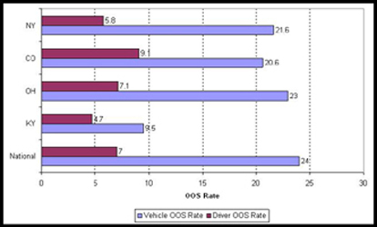
Scenario RE-1a examines the number of crashes avoided if Kentucky's vehicle and driver OOS rates were on par with national estimates. It is presented here to illustrate the increase in the number of crashes, injuries, and fatalities avoided if OOS rates in Kentucky were higher. However, for purposes of this crash avoidance analysis, scenario RE-1 (using Kentucky's current OOS rates) serves as the baseline when comparing results across scenarios.
Scenario RE-1a: Pre-ISSES/CVISN Using National OOS Rates
The calculation of crashes avoided in this scenario is very similar to the previous calculation, except that national OOS rates for vehicle and drivers based on actual inspections are used.
Using national OOS estimates from 2005, 24 percent of the 44,142 vehicle inspections would result in OOS orders. From Equation (5), the predicted number of crashes avoided due to vehicle OOS orders is equal to
![]() (11)
(11)
Similarly, 7 percent of 86,028 driver inspections would result in an OOS order leading to
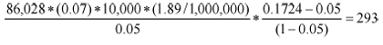 (12)
(12)
crashes avoided.
Applying the 51 percent adjustment factor used under random selection, the estimated number of crashes avoided is 65 + 0.51*293 = 214. The corresponding numbers of injuries and fatalities avoided are 55 and 3, respectively.
As expected, the number of crashes, injuries, and fatalities prevented would be larger under this scenario, which brings Kentucky's OOS rates more in line with national averages. Also, the estimated number of crashes avoided under normal (pre-ISSES/CVISN) inspection practices is about 17 percent higher (214 versus 183) than the number that would be avoided under random selection of vehicles.
Scenario RE-2: Mainline Electronic Screening Based on ISS Score
Currently, 32 states use some form of mainline electronic screening as part of their roadside enforcement. However, even in these states, carrier enrollment in electronic screening is not sufficient to demonstrate any significant impacts on the inspection selection process. Therefore, to illustrate what could happen, the impact of using electronic screening was simulated using results from the field study at the Laurel County station. An analysis was performed under the scenario that: (1) Kentucky deploys electronic screening at all major inspection sites; and (2) all of the motor carriers with ISS ratings in the low- or medium-risk categories (representing approximately 60 percent of all trucks) choose to enroll in the electronic screening program.
Under this scenario, enforcement officials could choose to let the low- and medium-risk vehicles bypass the inspection site and focus all of their efforts on inspecting high risk carriers and carriers with insufficient safety data. It is assumed that current inspection methods involving manual pre-screening (i.e., visual inspection and inspector experience/judgment) are used, as in scenario RE-1, on the 40 percent of trucks that are not allowed to bypass the inspection site. Section 6.5.2 presented an analysis demonstrating that, under this scenario, the number of OOS orders would increase by 50 percent compared to the average number that would be achieved under current inspection practices. It is assumed that the 50-percent increase in OOS orders would apply equally to vehicle OOS orders and driver OOS orders, therefore translating into a 50-percent increase in the number of crashes avoided.
From here, the calculation of the numbers of crashes, injuries, and fatalities avoided under scenario RE-2 is straightforward. With a 50 percent increase in OOS orders, the number of crashes that can be avoided under RE-2 is 1.50 * 126=189. This represents an increase of 63 crashes avoided compared to the baseline scenario. The corresponding number of injuries avoided is 49 (a difference of 16), and the number of deaths avoided is 2 (no change from RE-1).
Scenario RE-3: Electronic Screening based on Kentucky OOS Rate Inspection Selection Algorithm
To illustrate what could happen if the Kentucky OOS Rate Inspection Selection Algorithm were utilized at all Kentucky inspection sites, an analysis was performed under the scenario that: (1) the ISSES is able to accurately identify each truck that traversed the station; (2) the ISSES is linked with the Kentucky Clearinghouse so that the carrier's vehicle and driver OOS rates could be obtained; and (3) the algorithm is applied to identify trucks for possible inspection. In this scenario, those trucks with transponders are subject to the same algorithm already built into NORPASS as it is programmed to function in Kentucky.
Under this scenario, enforcement officials would only be concerned with trucks that were selected for possible inspection while other trucks were allowed to continue back to the mainline. In most cases, the number of trucks identified by the algorithm are too large for all of them to be inspected. As a result, enforcement officials would select vehicles to inspect from this pool of kicked out trucks.
Table 6-17 in Section 6.5.2 presented an analysis demonstrating that, under this scenario, the number of OOS orders would increase by 80 percent compared to the average number that would be achieved under scenario RE-1. It is assumed that the 80-percent increase in OOS orders would apply equally to vehicle OOS orders and driver OOS orders, therefore translating into an 80-percent increase in the number of crashes avoided. With an 80-percent increase in OOS orders, the number of crashes that can be avoided under RE-3 is 1.80 * 126=227. This represents an increase of 101 crashes avoided compared to the baseline scenario. The corresponding number of injuries avoided is 59 (a difference of 26), and the number of deaths avoided is 3 (a difference of 1).
Scenario RE-4: Electronic Screening based on high vehicle and/or driver OOS rates
In this scenario, the state utilizes the ISSES and/or electronic screening to screen all vehicles based on the vehicle and driver OOS rates of the carrier. This scenario is based on the premise that only trucks with the highest OOS rates are candidates for inspection while other vehicles are allowed to continue on the mainline.
Table 6-22 shows the three levels of threshold values for both the vehicle and driver OOS rate safety index. These trucks inspected during this 32.5-month timeframe were used as a proxy for the truck traffic population in Kentucky. The high threshold for the vehicle OOS rate index is 50%. This means that roughly 5% of the truck traffic has a vehicle OOS rate at or above 50%. The high threshold level would be used to pull in only the top 5% of vehicles in situations where a smaller number of inspectors were on duty. If more inspectors are available, a lower threshold can be used to pull more trucks into the station. The medium and low threshold values for the vehicle OOS rate safety index are 38.1% and 25.0%, respectively. The high, medium, and low thresholds for driver OOS rates are 22.2%, 16.7%, and 10.7%, respectively.
| Percent Selected for Inspection | Safety Index Threshold | |
|---|---|---|
| Carrier's Vehicle OOS Rate | Carrier's Driver OOS Rate | |
5% |
50.0% |
22.2% |
10% |
38.1% |
16.7% |
25% |
25.0% |
10.7% |
To use Equation (5) to estimate the number of crashes that would be prevented, a probit regression model was used to estimate the probability of an OOS violation among vehicles at or above each value of the index threshold. This probability represents the term P(V|Inspection) in Equation (5), namely the probability of finding an OOS violation given the truck was inspected with an index value above the threshold. By plugging the three threshold rates into the equation and solving for p, the probability of a violation given an inspection can be calculated for each level of the safety index. These probabilities are provided in Table 6-23 alongside the threshold values.
| Percent Selected for Inspection | Carrier Vehicle OOS Rate | Carrier Driver OOS Rate | ||
|---|---|---|---|---|
| Threshold | P(V|Inspection) | Threshold | P(V|Inspection) | |
5% |
50.0% |
0.26 |
22.2% |
0.11 |
10% |
38.1% |
0.17 |
16.7% |
0.08 |
25% |
25.0% |
0.10 |
10.7% |
0.05 |
From Equation (5), the number of crashes that are avoided due to vehicle OOS orders when the highest 5 percent of trucks in terms of vehicle OOS rate are brought into the station for inspection is equal to
![]() (13)
(13)
Similarly, 11 percent of the 86,028 driver inspections would result in an OOS order leading to
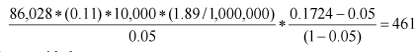 (14)
(14)
crashes avoided.
Applying the 51 percent adjustment factor used under the other scenarios, the estimated number of crashes avoided is 71 + 0.51*461 = 306. The corresponding numbers of injuries and fatalities avoided are 79 and 4, respectively.
The calculation for the number of crashes avoided using the medium (top 10 percent) and low (top 25 percent) threshold values is similar and not shown. Rather, the number of crashes, injuries and fatalities avoided under all three threshold levels is presented in Table 6-24.
| Percent Selected for Inspection | Number of Safety Events | ||
|---|---|---|---|
| Crashes | Injuries | Fatalities | |
5% |
306 |
79 |
4 |
10% |
217 |
56 |
3 |
25% |
134 |
35 |
2 |
As expected, the results for scenario RE-4 (above) and for scenarios RE-5 and RE-6 (presented below) indicate that the higher the threshold value for the safety index (i.e., with fewer but higher-risk trucks chosen for inspection), the more crashes, injuries, and fatalities can be avoided as a result of inspecting the same number of trucks. If a state has a low volume of truck traffic or extra inspectors available at a given site, however, officials might choose a lower threshold (e.g., top 10 percent or top 25 percent) to increase the total number of trucks available for inspection. The lower thresholds (10 percent and 25 percent) are shown partly to illustrate the effects of a state choosing to calibrate its threshold to better match the volume of truck traffic and the available inspection resources at a given site. For example, suppose an inspection site sees 2,000 trucks per day traverse the station during normal inspection hours. If the highest threshold value (5 percent) is used, about 100 trucks would be pulled out for inspection per day. Assume for purposes of illustration that 100 trucks is a normal volume of daily inspections at that station. If the state were to assign extra inspectors to that station, they might be underutilized if only 100 trucks were pulled in for inspection. In this case, it might be advantageous for the state to use a lower threshold level in an effort to inspect more than 100 trucks per day. More total inspections would be performed, compared to the number using the 5 percent threshold value. As noted, the figures in Table 6-24 show the safety benefits achieved based on a constant number of inspections (i.e., those performed statewide in Kentucky in 2005). If a state has the resources to inspect more trucks, even under a lower threshold level, the relative safety benefits would be expected to rise. Such benefits, however, were not quantified in this analysis.
The high threshold level represents an increase of 180 crashes avoided compared to the baseline scenario (RE-1). Also, about 46 more injuries and 2 more fatalities are avoided under this scenario.
Scenario RE-5: Electronic screening based on high driver or brake violation rate
This scenario is similar to RE-4 in that the state utilizes the ISSES and/or electronic screening to screen all vehicles at all major inspection sites based on a safety index. This scenario differs from RE-4 in that vehicles are screened on their brake violation rate as opposed to their overall vehicle OOS rate in an attempt to catch those vehicles that have a violation that has a higher relative risk for crash. Brake violation rates are defined as the number of brake violations for the carrier in the past 30 months divided by the number of vehicle inspections in the past 30 months.
Table 6-25 shows the three levels of threshold values for both the brake violation rate and driver OOS rate safety index. The high threshold for the brake violation rate index is 1.07. This means that roughly 5 percent of the truck traffic has a brake violation rate at or above 1.07. The high threshold level would be used to pull in only the top 5 percent of vehicles in situations where a smaller number of inspectors were on duty. If more inspectors are available, a lower threshold can be used to pull more trucks into the station. The medium and low threshold values for the brake violation rate safety index are 0.81 and 0.50, respectively. Note that the thresholds for the driver OOS rate are the same as in RE-4.
| Percent Selected for Inspection | Safety Index Threshold | |
|---|---|---|
| Brake Violation Rate | Driver OOS Rate | |
5% |
1.07 |
22.2% |
10% |
0.81 |
16.7% |
25% |
0.50 |
10.7% |
To use Equation (5) to estimate the number of crashes that would be prevented, a probit regression model was used to estimate the probability of an OOS violation among vehicles at or above each value of the index threshold. This probability represents the term P(V|Inspection) in Equation (5). By plugging the three threshold rates into the equation and solving for p, the probability of a brake-related OOS violation given an inspection can be calculated for each level of brake violation rate. These brake-related probabilities are provided in Table 6-26 along with the probabilities associated with the driver OOS rate index originally presented in RE-4.
| Percent Selected for Inspection | Brake Violation Rate | Driver OOS Rate | ||
|---|---|---|---|---|
| Threshold | P(V|Inspection) | Threshold | P(V|Inspection) | |
5% |
1.07 |
0.14 |
22.2% |
0.11 |
10% |
0.81 |
0.11 |
16.7% |
0.08 |
25% |
0.50 |
0.07 |
10.7% |
0.05 |
From Equation (5), the number of crashes that are avoided due to brake-related OOS orders when the highest 5 percent of trucks in terms of brake violation rate are brought into the station for inspection is equal to
![]() (15)
(15)
This estimated number of crashes avoided is conservative. The calculation is based in part on the probability of finding a brake-related OOS condition in the population. According to the National Fleet Safety Study (NFSS) performed in 1996, 14 percent of VMT are with brake-related OOS conditions (Star 1997). In reality, an inspector is going to place a truck OOS if any vehicle OOS violation is found, not just a brake-related one. Thus, the numbers of crashes, injuries, and fatalities reported under scenario RE-5 are conservative.
Eleven percent of the 86,028 driver inspections would result in a driver OOS order leading to
![]() (16)
(16)
crashes avoided.
Note that these two numbers cannot be added to get the total number of crashes avoided because there is some overlap in brake and driver OOS orders. As reported in RE-0, the TFSS found that 49 percent of the inspections that found at least one driver OOS violation also found at least one vehicle OOS violation (USDOT 2006b). Furthermore, the study found that brake OOS violations represent 42 percent of all vehicle OOS violations. As a result, about 21 percent (0.49*0.42) of the inspections that found at least one driver OOS violation also found at least one brake OOS violation. Because the impact of brake OOS orders is greater than the impact of driver OOS orders, the number of crashes avoided combined over brake-related and driver OOS orders can be determined by adding (a) the number of crashes avoided due to brake-related OOS orders and (b) 79 percent of the crashes avoided due to driver OOS orders. Thus, the total number of crashes avoided annually in Kentucky would be 112 + (0.79*461) = 476. The corresponding numbers of injuries and fatalities avoided are 123 and 6, respectively.
The calculation for the number of crashes avoided using the medium (top 10 percent) and low (top 25 percent) threshold values is similar and not shown. Rather, the number of crashes, injuries and fatalities avoided under all three threshold levels is presented in Table 6-27.
| Percent Selected for Inspection |
Number of Safety Events Avoided |
||
|---|---|---|---|
| Crashes |
Injuries |
Fatalities |
|
5% |
476 |
123 |
6 |
10% |
353 |
91 |
4 |
25% |
221 |
57 |
3 |
As described above for RE-4, the results for RE-5 indicate that the higher the threshold value for the safety index, the more crashes, injuries, and fatalities can be avoided as a result of inspecting the same number of trucks with higher violation or OOS rates.
The high threshold level represents an increase of 350 crashes avoided compared to the baseline scenario. Also, about 90 more injuries and 4 more fatalities are avoided under this scenario.
RE-6: Electronic screening based on infrared screening and high driver OOS Violation Rate
Roadside scenario RE-6 is similar to RE-5 in that it focuses on identifying vehicles that have brake and/or driver OOS violations (violations with high relative crash risk). Where RE-6 differs from RE-5 is that brake violations are screened via IR technology rather than the carrier's brake violation rate. Prior research conducted in 2000 for FMCSA on evaluating an IR imaging and video package, IRISystem, found that the percentage of vehicles placed OOS due to brake violations after IRISystem screening was 47.2%. This figure is used as an estimate for the probability of a brake violation given that an inspection occurred, [P(V|Inspection)].
From Equation (5), the number of crashes that are avoided due to brake OOS violations when the thermal imaging system is used to select vehicles for inspection is equal to
![]() (17)
(17)
This estimated number of crashes avoided is conservative. The calculation is based in part on the probability of finding a brake-related OOS condition in the population. In reality, an inspector is going to place a truck OOS if any vehicle OOS violation is found, not just a brake-related one. Thus, the numbers of crashes, injuries, and fatalities reported under scenario RE-6 are conservative.
The number of crashes that are avoided due to driver OOS violations when the highest 5 percent of trucks in terms of driver OOS rate are brought into the station for inspection is equal to
![]() (18)
(18)
Applying the 79 percent adjustment factor used in RE-5, the estimated number of crashes avoided is 379 + 0.79*476 = 755. The corresponding numbers of injuries and fatalities avoided are 196 and 9, respectively.
The calculation for the number of crashes avoided using the medium (top 10 percent) and low (top 25 percent) threshold values for the driver OOS rate index is similar and not shown. Rather, the number of crashes, injuries, and fatalities avoided under all three threshold levels is presented in Table 6-28. While the driver OOS rate threshold change for each of the high, medium, and low, levels, the brake OOS rate of 47.2% when using IR technology remains unchanged.
| Threshold Level for Driver OOS Rate |
Number of Safety Events Avoided |
||
|---|---|---|---|
| Crashes |
Injuries |
Fatalities |
|
High (Top 5%) |
755 |
196 |
9 |
Medium (Top 10%) |
644 |
167 |
8 |
Low (Top 25%) |
544 |
141 |
7 |
Using the high threshold level for driver OOS rate represents an increase of 629 crashes avoided compared to the baseline scenario. Also, about 163 more injuries and 7 more fatalities are avoided under this scenario.
As discussed above for RE-4, the results for RE-6 indicate that the higher the threshold value for the safety index, the more crashes, injuries, and fatalities can be avoided as a result of inspecting the same number of trucks with higher values of the safety index.
6.6.4 Summary of Results
Table 6-29 summarizes the major results of this safety benefits analysis. According to the model, current roadside enforcement strategies (RE-1) are responsible for avoiding 126 truck-related crashes, which represents about 4.4 percent of the 2,853 crashes in Kentucky that occur annually, based on 2005 crash statistics. Furthermore, it is estimated that current roadside enforcement activities are responsible for preventing 33 injuries and 2 deaths. The safety benefits realized increases with each scenario RE-2 through RE-6. The maximum benefit is achieved with RE-6, where 755 crashes are avoided if the top 5 percent of vehicles in terms of driver OOS violations are inspected in conjunction with IR screening. This implies that about 26 percent of Kentucky's 2,853 annual truck-related crashes could be avoided under RE-6. In reality, this figure is an overestimate, because national crash rates were used in the safety benefit calculations, because reliable crash rates for Kentucky were not available.
To put the crash avoidance numbers into context, consider that the number of large trucks involved in crashes in Kentucky (2,853) is low relative to the 441,000 large trucks involved in crashes nationally, representing only 0.6 percent of national crashes. Also, the percent of Kentucky crashes relative to the number of inspections performed in Kentucky is about 3.3 percent. Comparatively, the national rate of crashes relative to the number of inspections is about 16 percent. Therefore, relative to the number of inspections, Kentucky's crash rate is smaller than the national crash rate. The exact reason for this is unknown, but possible explanations include a lower volume of traffic in Kentucky, less congested highways, or a smaller number of large cities.
Recalculating the safety benefits achieved when the national number of vehicle and driver inspections in 2005 is used instead of Kentucky inspection figures in Equation (5) finds that implementing RE-6 avoids about 6.5 percent of all national crashes. This figure makes more sense in the context of the number of total crashes.
It is not possible to know the exact percentage of crashes caused by driver or brake OOS violations. However, as discussed earlier, there is a 12.2 percent increase in relative crash risk for driver OOS violations, a 4.4 percent increase in crash risk for vehicle violations, and a 7.7 percent increase in crash risk for brake OOS violations. Since a vehicle could have more than one type of violation, the three crash risk figures cannot be added to obtain the total increase in crash risk. However, these figures suggest that if there were no driver or brake OOS violations present in the population, no more than about 20 percent of crashes could be avoided. This is the maximum possible benefit if all OOS violations were removed from trucks traveling on the road. This fact helps to put the Kentucky results into context and to provide an upper bound on the crash avoidance numbers for Kentucky.
| Scenario | Description | Numbers of Safety Events Avoided1 | Additional2 Safety Events Avoided (ISSES/CVISN Benefit) | |||||
|---|---|---|---|---|---|---|---|---|
| Crashes | Injuries | Fatalities | Crashes | Injuries | Fatalities | |||
RE-0 |
Random Selection |
183 |
47 |
2 |
||||
RE-1 |
Baseline - Pre ISSES/CVISN Using Kentucky OOS Rates |
126 |
33 |
2 |
||||
RE-1a |
Pre ISSES/CVISN Using National OOS Rates |
214 |
55 |
3 |
||||
RE-2 |
Mainline Electronic Screening Based on ISS Score |
189 |
49 |
2 |
63 |
16 |
0 |
|
RE-3 |
Electronic Screening based on Kentucky OOS Rate Inspection Selection Algorithm |
227 |
59 |
3 |
101 |
26 |
1 |
|
RE-4 |
Electronic Screening based on high vehicle and/or driver OOS rates3 |
5% 10% 25% |
306 217 134 |
79 56 35 |
4 3 2 |
180 91 8 |
46 23 2 |
2 1 0 |
RE-5 |
Electronic screening based on high driver or brake violation rates3 |
5% 10% 25% |
476 353 221 |
123 91 57 |
6 4 3 |
350 227 95 |
90 58 24 |
4 2 1 |
RE-6 |
Electronic screening based on infrared screening and high driver OOS violation rate3 |
5% 10% 25% |
755 644 544 |
196 167 141 |
9 8 7 |
629 518 418 |
163 134 108 |
7 6 5 |
2 Compared to baseline scenario (RE-1).
3Safety Benefits shown for strategies RE-4, RE-5, and RE-6 are dependent on the percentage of the truck population selected for inspection (top 5%, 10%, or 25% in terms of risk).
6.7 Credentialing Data
This section covers one additional data source that could potentially be used to help inspectors in their roadside enforcement decisions. This section assesses the usefulness of a carrier's credentialing status relative to their safety information in identifying high-risk trucks. To this point, most of the focus on data related to vehicles and carriers presented in this report has been related to safety. The goal was to determine if there exists a strong link between a carrier's credentialing status and their safety risk. Some credentialing information is available in federal and state databases. The ISSES, when integrated with these data sources, will allow inspectors real-time, instant access to credentialing data.
Although some credentialing data is present in the Kentucky Clearinghouse database, it is limited in terms of the number of carriers that have information as well as the number of credentials where information is available. This is a direct result of the Clearinghouse not being fully linked to any federal data source such as SAFER. Because of these limitations, credentialing data were left out of the scenarios presented in Section 6.6 and instead are presented separately in this section. Table 6-30 lists the most common credentials needed to operate in Kentucky for which information is available in the Clearinghouse.
| Credential | Explanation |
|---|---|
International Fuel Tax Agreement (IFTA) |
Fuel tax agreement for carriers engaged in interstate operations |
International Registration Plan (IRP) |
Registration for carriers engaged in interstate operations |
Weight Distance Tax (WDT) |
Mileage tax for carriers operating within Kentucky |
Kentucky Intrastate Tax (KIT) |
Fuel tax for intrastate carriers |
Extended Weight [Coal] Decal (EWD) |
Permit for companies hauling coal on state maintained highways |
Kentucky Highway Use (KYU) License |
Used to report mileage tax |
One example of the limited Clearinghouse credentialing data is that while IFTA information is available for all Kentucky based carriers where IFTA is applicable, information from other states is scarce. Kentucky does interface with the IFTA Clearinghouse to capture IFTA revocation data from carriers in other states; however the IFTA information from other states needs to include the USDOT number in order to be processed by Kentucky because the Kentucky Clearinghouse is a carrier-based system. Since a large amount of information from other states is not processed in the IFTA Clearinghouse by USDOT number, the Kentucky Clearinghouse gets limited IFTA information from other states. Over 31% of all carriers with available IFTA information in the Kentucky Clearinghouse are based in Kentucky.
Also, IRP information is strictly limited to Kentucky-based carriers in the Kentucky Clearinghouse. According to representatives of the KTC, the IRP Clearinghouse is currently geared more toward proper recording of registration fund transfers and does not have a strong real-time revocation system. Thus, the Kentucky Clearinghouse does not have IRP information for non-Kentucky carriers.
All carriers traveling in Kentucky are subject to the weight distance tax (WDT) as well as the Kentucky Highway Use License displayed via the Kentucky Use (KYU) number on trucks that operate in the state. Since information for these taxes is housed in a Kentucky state database, the Kentucky Clearinghouse contains WDT and KYU status on a larger number of carriers (both based within and outside of Kentucky). The Extended Weight Decal (EWD) Permit is not used as much as some other credentials and, as such, not a lot of carriers in the Clearinghouse have EWD information. The Kentucky Intrastate Tax is for intrastate carriers only and is obtained from another Kentucky database.
One objective of the inspection efficiency portion of the evaluation was to determine if having access to a carrier's credentialing status would provide new information beyond safety information, such as ISS scores and OOS rates, to an inspector to help him or her select high-risk trucks for inspection. Unfortunately, due to the limits in the amount of data available in the Kentucky Clearinghouse, a complete analysis could not be conducted. However, a few simple analyses were performed to show the relationship between a carrier's risk rating as defined by their ISS score and their credentialing status using IFTA and WDT as examples.
Table 6-31 illustrates the results using a carrier's IFTA status. For each carrier in the Kentucky Clearinghouse where information on IFTA was available, information was captured to determine if the carrier was in good standing with regard to IFTA. In addition, the USDOT number for each of these carriers was cross referenced with SAFER to obtain the carrier's ISS score. The ISS score was used to assign the carrier to one of five risk categories: high-risk, medium-risk, low-risk, insufficient data, or unknown. The carrier risk ratings are the same as presented in Section 6.4. Carriers having insufficient or unknown data were excluded from this analysis. Of the 2,558 carriers in good IFTA standing, 25 percent were considered high-risk as compared to 32 percent of the 1,510 carriers not in good standing that were high-risk. The percentage of medium-risk carriers not in good IFTA standing was also higher (33 percent) than those carriers in good standing (26 percent).
| Credentials in Good Standing | Credentials NOT in Good Standing | |||
|---|---|---|---|---|
| Risk Level | Number of Carriers | Percent | Number of Carriers | Percent |
High |
632 |
25% |
1,510 |
32% |
Medium |
664 |
26% |
1,546 |
33% |
Low |
1,262 |
49% |
1,612 |
35% |
Total |
2,558 |
100% |
4,668 |
100% |
Table 6-32 shows similar results when carrier risk rating is compared to WDT status. Thirty-eight percent of carriers not in good WDT standing were considered high-risk versus 24 percent of carriers in good WDT standing. The percentage of medium-risk carriers with not in good WDT standing was slightly higher (31 percent) than those carriers in good standing (29 percent).
| Credentials in Good Standing | Credentials NOT in Good Standing | |||
|---|---|---|---|---|
| Risk Level | Number of Carriers | Percent | Number of Carriers | Percent |
High |
50,481 |
24% |
3,844 |
38% |
Medium |
61,137 |
29% |
3,222 |
31% |
Low |
98,458 |
47% |
3,166 |
31% |
Total |
210,076 |
100% |
10,232 |
100% |
Both Tables 6-31 and 6-32 illustrate that there appears to be a loose correlation with a carrier's credentialing status and the company's safety risk rating. However, due to the data limitations in the Kentucky Clearinghouse, a more thorough and complete analysis is needed to fully understand and assess the relationship between a carrier's safety and credentialing information.
Also, Kentucky is currently in the process of implementing their Commercial Vehicle Information Exchange Window (CVIEW). Testing was being finalized in October and November of 2007. This CVIEW, unlike the Kentucky Clearinghouse, will be directly linked to federal and state databases such as SAFER, License and Insurance (L&I), and MCMIS. As such, inspectors at the roadside will have access to timelier and larger quantities of data, including credentialing, for use in roadside enforcement.
2The IRISystem technology was purchased by IIS (the vendor for the ISSES technology under evaluation) in 2003. IIS continues to manufacture IRISystem vans, and the IRISystem designer participates in all of IIS's thermal imaging applications.
3The term "electronic screening" is defined, for purposes of this study, as using any computer-based, real-time information source to aid in selecting trucks for inspection, whether the truck carries a transponder or not, and whether the screening occurs at mainline or ramp/sorter-lane speeds. Further details are provided in Section 6.6.2 below.
4Although not broken out separately for analysis in this evaluation, as a point of reference, the following is a description of the population of 93 trucks chosen for inspection during the two-week field study at Laurel northbound station. About 46 percent of the trucks were classified as high-risk. This is higher than the 34 percent of all trucks inspected during the 32.5-month period, as shown in Table 6-10 below. Although the exact reason for the difference is unknown, possible explanations include variations in inspector skills and methods, time of day, and changing weather conditions between the longer and shorter time periods of analysis. Factors such as these could have an impact on the truck population or the inspection efficiency of a particular site. By contrast, of these 93 trucks inspected, five had an OOS violation (four were driver-related and one was vehicle-related). This OOS rate of 5.4 percent was, incidentally, lower than the 13.6 percent statewide historical OOS rate.
5 Although more current crash statistics are available, the safety benefits analysis is performed using a baseline year of 2005 because that was the last year for which complete data were available from all of the relevant sources.