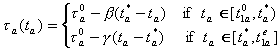
and ending
at
and ending
at  . Whenever a person does not
arrive on time or leave on time, a positive schedule delay is incurred.
. Whenever a person does not
arrive on time or leave on time, a positive schedule delay is incurred.
In an effort to reduce queuing delays at toll booths, many toll facilities
now only collect the toll in one direction. In fact, many older facilities have
removed existing toll plazas/barriers and many newer facilities are only
constructing a single plaza/barrier. Unfortunately, this makes it difficult to
charge time-varying tolls in both directions even with electronic toll
collection since it is unlikely that all vehicles will be equipped with this
technology. This paper explores how this difficulty might be overcome.
When toll facilities were first constructed and for many years thereafter it
was common to collect tolls from vehicles traveling in both directions. Indeed,
this approach is quite natural since in many cases it is not necessary to use
the same facility in both directions. Unfortunately, as the amount of traffic on
these facilities increased, so did the amount of time spent in queues waiting to
pay the toll. In an effort to reduce the amount of time wasted in queues (and
reduce the cost of collecting the tolls) many facilities began collecting tolls
in one direction only, charging the round-trip toll in that direction. This
policy has worked so well that many facilities removed the second (unnecessary)
toll plaza/barrier (e.g., the tunnels and bridges connecting New York and New
Jersey, the Sumner/Callahan Tunnels in Boston). In addition, many newer
facilities are being constructed with a single toll plaza/barrier (i.e., in one
direction only).
Unfortunately, while this practice does seem to have worked well in the past,
it has been argued that it makes it very difficult to implement some kinds of
pricing policies. Recall that toll policies can be used in different ways to
influence the decision to travel, destination choice, mode choice, route choice
and departure-time choice (1). When tolls can only be collected in one
direction it becomes impossible to use time-varying tolls to influence the
departure-time choices of people traveling in both directions.
At first glance, it would seem that this problem could easily be overcome
using electronic toll collection (ETC) (2). However, since it is
virtually impossible (at this point in time anyway) to require that all vehicles
make use of ETC, it is not immediately clear that this technological fix is
workable.
In this paper we will discuss how ETC may make it possible to implement AM
and PM congestion pricing even when there is a toll plaza/barrier in only one
direction and all vehicles are not required to make use of ETC. In addition, we
will discuss how this approach may correct some of the adverse distributional
impacts of congestion pricing, eliminate the need to redistribute the toll
revenues, and allay the fears [see, for example, Higgins (3)] that
congestion pricing is unfair, discriminatory, regressive, coercive and
anti-business. The approach we suggest for achieving these goals makes use of
both time-varying tolls and time-varying subsidies, as discussed by Bernstein
(4).
To illustrate the potential benefits of this approach we extend the
traditional one-directional model (5-9) so that it can be used to
study AM/PM commuting. As it turns out, this is not equivalent to simply
"considering the AM peak twice" for several reasons. First, as discussed by
Fargier (10), the commuting schedule in the evening is different from
that in the morning(e.g., there is no desired arrival time for the PM trip).
Second, work-to-home trips often involve secondary trips (e.g., shopping,
dinner) making the origin/destination, route and departure-time choices more
irregular. Third, AM and PM decisions are not independent (i.e., the decision
you make in the AM affects the one you make in the PM).
This paper begins with a description of the model itself. It then considers
AM/PM tolling with one plaza when there is only one relevant route. Next, it
considers the implications of AM/PM tolling on multiple routes. Finally, it
considers a variety of implementation details and concludes with a discussion of
future research.
In order to get some insight into commuters' route and departure-time
decisions, we will work with a model with N homogenous commuters
traveling between home and work. The decisions for a commuter are to choose both
their AM and PM departure-times and routes in order to minimize their round-trip
travel cost. The travel cost is composed of the total travel time and the
schedule delay (plus tolls if any).
C=a[T(ta)+T(tp)]+(Fa+ Fp)+(a+p) (1)
where C is the travel cost; T(ta) and T(tp) are the
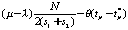
travel times for the AM and PM trips; Faand Fp are the AM and PM schedule delays; a and
p are the AM and PM tolls (or subsidies); and a is the dollar value of travel time. There is a desired work
schedule starting from and ending
at . Whenever a person does not
arrive on time or leave on time, a positive schedule delay is incurred.
Of course, the AM and PM schedule delays may or may not be correlated. For
example, suppose people must work exactly eight hours every day. This implies
that the departure-time choices for the morning and evening are perfectly
correlated (i.e., a person that arrived 20 minutes late in the morning must
leave 20 minutes late in evening). However, this situation rarely occurs. In
most cases, the eight hour work-day can only be viewed as a loose constraint.
That is, the departure time decisions for the AM and PM are not always perfectly
dependent. In fact, in some cases they are independent. For example, some people
have fixed start and end times for their work-day. Hence, even if they arrive
after 9:00AM they do not get compensated for working after 5:00PM. For
simplicity, here we assume that the schedule delays are completely independent.
The AM schedule delay depends only on when the commuter arrives at work in the
morning and the PM schedule delay depends only on when he/she leaves from work
in the evening. Therefore the schedule delays are given by:
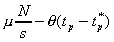
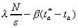
Fa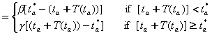 (2)
(2)
and
Fp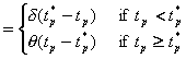 (3)
(3)
where b and g denote the
dollar penalties for early and late arrivals to work, and d and q are the dollar penalties for
early and late leaves from work. In addition, following notations for some
important time points are introduced:  -beginning of peak (j=a, p),
  -ending of peak(j=a, p) and
  -AM departure time to arrive at work on
time[i.e.,
-AM departure time to arrive at work on
time[i.e.,  ].
].
We also assume that the time needed to travel in each direction can be
modeled as a deterministic queuing process in which:
T(tj)=D(tj)/s, j=a, p (4)
where s is the service rate (road capacity) and D(tj) is the queue length at time tj. This approach is believed to represent actual travel time functions fairly well. Finally, we assume that in equilibrium no individual has any incentive to change his/her departure-time or route choice. The equilibrium departure rates that arise from such a model are given by:
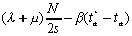
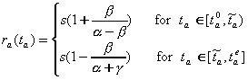 (5)
(5)
and
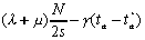
 (6)
(6)
We first assume that there is only one route between work and home, and that
there is only one toll plaza (in the AM inbound direction). As shown in the
Appendix, both the AM and PM departure rates are greater than the service rate
before the desired departure time and smaller than the service rate after that
time. Thus, the queues in both directions reach their maximums at the desired
departure times. With these results, we can now consider how to construct
pricing schemes that eliminate congestion in both directions. As it turns out,
there are at least three optimal pricing schemes, each of which is discussed in
detail below. The analytical expressions for these pricing schemes are given in
Table 1.
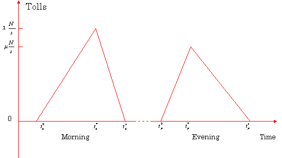
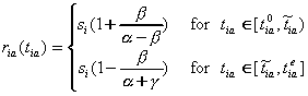
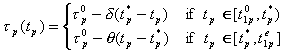
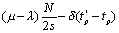
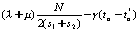
The first scheme is a traditional one in which commuters are charged positive
tolls for both their AM and PM trips. The optimal toll structure is shown in
Figure 1. Here  and
and . The AM peak starts at
  and ends at
  and the PM peak starts at
  and ends at
  .
.
Under this scheme, the tolls are zero at the beginnings and the ends of AM
and PM rush hours, and they reach the peaks at the scheduled arrival time  , and the scheduled departure time
  . The merit of this pricing scheme is
that it only charges commuters (i.e., people who travel during the rush hours);
non-commuters (i.e., people who travel outside of the rush hours) can continue
to enjoy their trips free of charge in both directions.
. The merit of this pricing scheme is
that it only charges commuters (i.e., people who travel during the rush hours);
non-commuters (i.e., people who travel outside of the rush hours) can continue
to enjoy their trips free of charge in both directions.
Though in theory above pricing scheme can eliminate traffic congestion and
has some nice properties, in practice it is not the preferable approach for two
reasons. First, this type of scheme is subject to the criticisms that it is
unfair, discriminatory, regressive, coercive, and anti-business (3). The
average individual's share for this "tax" in above scheme is clearly greater
than zero and it increases as the peak duration becomes longer. It is not clear
how this toll revenue is redistributed to the society. Second, this scheme
requires two toll plazas, one in each direction, to collect the tolls. Note that
this problem cannot be overcome by electronic toll collection (ETC) unless all
vehicles are equipped since there would be no way to charge unequipped vehicles
without the toll plaza. Hence, there would be no way to influence their
behavior. In addition, equipped vehicles would pay higher tolls than unequipped
vehicles and hence would be encouraged to stop using ETC. It is clear that this
pricing scheme can not be implemented without two enforcement barriers no matter
whether there exists an ETC or not.
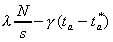
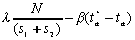
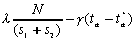
The second scheme is designed to consider the two practical requirements:
that there is no barrier for the PM outbound and that the toll revenue must be
zero. By imposing these two constraints, the drawbacks with previous scheme can
be eliminated. The method for incorporating these constraints is to impose
negative tolls (subsidies) on the PM outbound direction in which there is no
toll plaza. Such a pricing scheme with tolls and subsidies, which is still
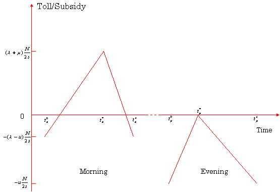
optimal, is drawn in Figure 2.
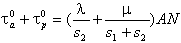
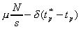
In figure 2, it is interesting to note that the AM toll can be positive or
negative depending on the parameters. If l>m, then
all commuters arrive before  and
after
and
after  will receive a subsidy and all
others have to pay a toll. However, if l
will receive a subsidy and all
others have to pay a toll. However, if l m, then all commuters must pay
positive tolls in the morning.
m, then all commuters must pay
positive tolls in the morning.
It is also interesting to note that the toll revenue collected in the morning
is redistributed to the commuters in the evening. It can be seen from Figure 2
that the total toll revenue is zero. Therefore there is no reason for people to
view this type of congestion pricing as a tax. More importantly, the PM subsidy
can be distributed without a toll plaza. Vehicles equipped with ETC will be able
to receive the subsidy and unequipped vehicles will not. Thus, this will
encourage people to participate the ETC systems.
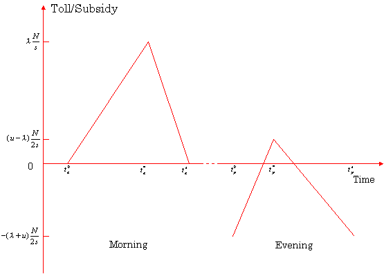
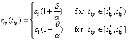
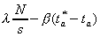
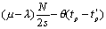
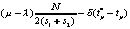
An alternative scheme that may also meet the requirements of zero toll
revenue and one barrier is illustrated in Figure 3. In this scheme, AM toll is
positive during the entire morning rush hours (a pure toll) and this would
simplify the toll collection for the AM trips. However the PM toll can either be
negative during the whole rush hour (a pure subsidy) or be negative in some
periods and positive in the others (a mixed toll and subsidy), depending on the
relationship among the parameters. If  , then PM toll is a pure subsidy
structure which is desirable. If, however, l<m, then
during any period between
, then PM toll is a pure subsidy
structure which is desirable. If, however, l<m, then
during any period between  and
and  a positive toll is charged.
Nevertheless, as can be seen in Figure 3, the total toll revenue is always zero
regardless the parameters.
a positive toll is charged.
Nevertheless, as can be seen in Figure 3, the total toll revenue is always zero
regardless the parameters.
Though in theory all three of the above pricing schemes are socially optimal,
scheme 1 is the most difficult to implement. However, it is worth considering
the pros and cons of schemes 2 and 3 in somewhat more detail. Depending upon the
parameters, either scheme 2 or scheme 3 must have a mixed toll/subsidy structure
for the same direction trips. In scheme 3, there might exist some periods during
which the PM tolls are positive but clearly such positive tolls can not be
collected without a toll plaza. On the other hand, though scheme 2 could be
operated from a purely technological standpoint, it introduces a
non-technological problem. Observe that under the condition of l>m, there are some periods in the AM and all the periods
in the PM during which commuters are actually being paid to use the road.
Therefore it is possible that a person can make money simply by traveling back
and forth during the subsidy periods. This means that scheme 2 can encourage
spurious trips (i.e., trips simply aimed at receiving subsidies). Though, as
discussed later, there may be some ways to discourage such spurious trips using
existing technologies, the incentive for such spurious trips should be kept as
low as possible. Observe that a pricing program with a pure toll for the AM
trips and a pure subsidy for the PM trips is implementable in our context. Such
a pure toll/subsidy program may also discourage spurious trips because the AM
toll may outweigh the PM subsidy.
It follows that if l<m, then scheme 2 should be
chosen; if, however, l>m, then scheme 3 should be
chosen. By this selection criterion, we can get a program with a pure toll for
the AM and a pure subsidy for the PM. When l=m, there
is no difference between scheme 2 and 3. Observe that this selection criterion
does not depend on the roadway condition (i.e., capacity). It is only determined
by how people value the schedule delay and thus it is applicable anywhere.
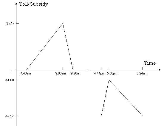
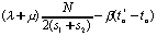
In order to illustrate these ideas we consider a numerical example. We assume
that  =9:00 AM,
  =5:00 PM, s=6000 vehicle/hour and N=10000
vehicles. For the shadow value parameters we use the oft-cited values for the AM
trips (11-12) a=$6.40, b=$3.90, g=$15.21. For the PM trips
we arbitrarily use d=g=$15.21,
and q=$3.00. Here q is assumed
to be smaller than b because people can participate in
secondary activities after work and before heading for home, such as shopping,
dining and other social activities. This possibility decreases the shadow value
of departing late (13).
=5:00 PM, s=6000 vehicle/hour and N=10000
vehicles. For the shadow value parameters we use the oft-cited values for the AM
trips (11-12) a=$6.40, b=$3.90, g=$15.21. For the PM trips
we arbitrarily use d=g=$15.21,
and q=$3.00. Here q is assumed
to be smaller than b because people can participate in
secondary activities after work and before heading for home, such as shopping,
dining and other social activities. This possibility decreases the shadow value
of departing late (13).
In this case, the rush hour lasts from 7:40AM to 9:20AM in the morning and
from 4:44PM to 6:24PM in the evening. Since l>m in
this example, scheme 3 is selected. As shown in Figure 4, the AM toll first
increases smoothly from zero dollar at 7:40AM, reaches the peak of $5.17 at
9:00AM and then falls to zero at 9:20AM. The PM subsidy begins with a maximum of
$4.17 at 4:44PM, falls to a minimum $1.00 at the 5:00PM, and then increases and
reaches the maximum again at 6:24PM.
We should compare our two-way work trip model with the one-way morning trip
model. Table 2 shows the average costs per commuter under four scenarios: no
toll, one-direction toll, two-directional tolls and two-directional
toll/subsidy. From this table, it is clear that one-directional tolling is not
efficient and can be improved (i.e., social savings increase from 27.7% to
50%).
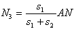
We now consider a network in which there are two parallel routes. Let the capacity at route 1 be s1 and the capacity at route 2 be s2. When there is no congestion pricing, the equilibrium departure rates can be shown as follows:
 i=1,
2 (7)
i=1,
2 (7)
and
 i=1,
2 (8)
i=1,
2 (8)
where i=1,2 is the route index. This result is similar to the single route
case. It can also be shown that the beginning and ending times of peaks for two
routes are the same:
 , and
, and  j=a, p
(9)
j=a, p
(9)
The route split between two routes is proportional to the ratio of the
capacities (s1/s2). This equilibrium split coincides with
the system optimum. The intuition behind is clear: the larger the road is, the
more people on that road.
This result seems to suggest that an optimal pricing scheme should not alter
the users' route choices since they are already optimal. However, this
observation may not be true in some cases when not all of the routes are priced.
Once some routes can not be priced, the best (i.e. system optimal) pricing
scheme may be not achievable. Instead, the second-best should be used. We now
consider AM/PM pricing for two cases: when both roads can be tolled and when one
must be left un-tolled.
In the first case we assume that both roads can be tolled. Specifically we
assume that there are two toll plazas in the AM inbound direction, one in each
road and there is no toll plaza in the PM outbound direction. Since there is no
toll plaza in the PM outbound, subsidies are used to price the evening traffic.
Analogous to the one route case, there are two alternative optimal schemes
combining tolls and subsidies, as given in Table 3. These two schemes are
completely analogous to scheme 2 and scheme 3 in the single route case except
that the service rate has been replaced by the summation of the two routes'
service rates. Again, in order to get a pure toll /subsidy scheme, the selection
between these two schemes depends on the parameter l
and m. It is also interesting to see that the
tolls or subsidies at two routes are always equal. Therefore the route split is
unaffected since the equilibrium split is optimal.
In this case, we can extend above results to multiple routes in parallel.
That is, they can be treated as one single route in which the capacity is the
summation of all routes. The road usage is proportional to the capacity
regardless pricing or not. The starting times and the durations of the
congestion are the same for all routes. Finally, the optimal time-varying tolls
are also the same for all roads during any time of the day.
The more common situation in the real world is the existence of a mixture of
tolled and un-tolled facilities. Therefore it is more important to study the
case in which one route can be tolled and the other can not be tolled. This may
result because it is either physically impossible or publicly unacceptable to
collect tolls on all facilities. More interestingly, this situation can also
represent the single route case in which there are two types of toll booths:
manual and ETC-only. The non-ETC lane and the ETC lane can be modeled as two
routes and the decisions on equipping ETC tags or not can be seen as the choices
between two different routes.
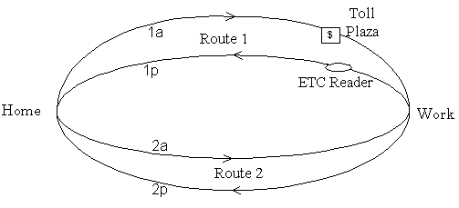
We assume, without loss of generality, that route 1 can be tolled and route 2
can not. As shown in Figure 5, there is one toll station located on route 1 AM
inbound and one ETC reader on the route 1 PM outbound. Since there is no
enforcement mechanism at the ETC reader, the only practical pricing scheme must
be an AM toll and PM subsidy scheme on route 1.
There are four possible paths for a round trip as follows:
Once a toll/subsidy pricing program is implemented, the costs for the these
four paths are described as follows. On path 1, a commuter must pay a toll in
the AM, receive a subsidy in the PM and incur no travel time cost on either
trips. On paths 2 and 3, there is no toll or subsidy but the travel time costs
are non-zeros. Though link 1p is used in the third path of (2a, 1p), there is no
subsidy received. As will be explained in the next section , only those persons
who have paid the tolls in the AM can receive subsidies. On path 4, a traveler
must pay a toll in the AM and receive no subsidy and spend some waiting time in
the PM. Thus this path will never be used because its cost is always greater
that the cost for path 1.
We treat the above route choices as if they are made hierarchically. The
first path's travelers are viewed as ETC users and the second and third paths'
travelers as non-ETC users. The commuters first have to decide to use the ETC
system or not. If they use ETC, then there is only one path. If not, they then
have to choose between the second path and the third path. This structure is
helpful because the congestion pricing scheme can only affect the first level
decision--ETC or non-ETC. The route split between the second path and the third
path for non-ETC users can not be influenced since they are not controllable.
Let numbers of people using these three paths be N1,
N2, and N3. The equilibrium
road usage can be derived as:
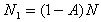 (10)
(10)
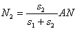 (11)
(11)
 (12)
(12)
where 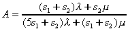 . The split between paths 2
and 3 are based on the road capacities while the split between ETC and non ETC
users depends on both the schedule delay parameters and the road capacities.
This equilibrium route split for the non-ETC users is not optimal for most
cases. This is because non-ETC users generate some unbalanced social costs on
two paths while users only pay the private costs, which are equal on two paths.
As a result, path 2 is overused if the capacity of route 1 is greater than the
capacity of route 2 and path 3 is overused if the capacity of route 1 is less
than the capacity of route 2. When the two routes have the same capacity, the
equilibrium route split will be optimal.
. The split between paths 2
and 3 are based on the road capacities while the split between ETC and non ETC
users depends on both the schedule delay parameters and the road capacities.
This equilibrium route split for the non-ETC users is not optimal for most
cases. This is because non-ETC users generate some unbalanced social costs on
two paths while users only pay the private costs, which are equal on two paths.
As a result, path 2 is overused if the capacity of route 1 is greater than the
capacity of route 2 and path 3 is overused if the capacity of route 1 is less
than the capacity of route 2. When the two routes have the same capacity, the
equilibrium route split will be optimal.
The average toll for a commuter using path 1 is
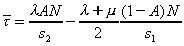 (13)
(13)
This toll revenue  can be
positive, zero or negative, depending on the relative capacities, (s1/s2), and the relative value of the schedule
delay parameters , (m/l).. For example, when the
capacity of route 1 is less than that of route 2 (i.e., s1<s2), the toll revenue is always negative
regardless the parameters of l and m. This also suggests that if we can only toll one road, we
should toll the bigger road because tolling on the smaller road will result in a
deficit. The optimal toll is given by:
can be
positive, zero or negative, depending on the relative capacities, (s1/s2), and the relative value of the schedule
delay parameters , (m/l).. For example, when the
capacity of route 1 is less than that of route 2 (i.e., s1<s2), the toll revenue is always negative
regardless the parameters of l and m. This also suggests that if we can only toll one road, we
should toll the bigger road because tolling on the smaller road will result in a
deficit. The optimal toll is given by:
 (14)
(14)
and
 (15)
(15)
where  and
and  are time-invariant uniform tolls and
they must satisfy:
are time-invariant uniform tolls and
they must satisfy:
 (16)
(16)
The pricing scheme for this case is sub-optimal in the sense that both the
route-split and the departure-rate for the non-ETC users are not optimal.
Because of the constraint of the optimal split between ETC and non-ETC, the toll
revenue can no long be set to zero.
There is one issue that needs to be addressed before a congestion pricing
program with both tolls and subsidies being implemented. Observe that in the PM
peak periods drivers are actually being paid to use the road. Hence, such a
program, if implemented incorrectly, could generate spurious trips in which
people drive simply to receive subsidies. Fortunately, there may exist some ways
to prevent such trips [see Bernstein (4) for details] in general.
In the specific setting considered here, the most interesting method to
discourage spurious trips is to give a subsidy only to those people who were
tolled in the other direction. In such a system, if a driver would like to
receive a subsidy in the evening peak, he/she would have to take an inbound trip
in the morning and pay a toll first. Therefore it is important to have the
information of the time and the route of the AM inbound trip for each vehicle
traveled in the subsidized roads. Such a task is easy to implemented using
existing technologies. In fact, almost all ETC systems could be modified to
record AM trips information and charge PM tolls (negative) based on the AM
activities. However, it may be advantageous to use an ETC system with read-write
capabilities rather than a read-only system. This is because with a read-write
system the information can be recorded in the vehicles themselves rather than in
a central computer. Thus there is no worry about "tracking" individual vehicles
and invading anyone's privacy. In such a system, whenever a vehicle arrives at
the subsidized outbound road in the PM, the reader/writer on the roadside first
checks the information stored in the in-vehicle unit. If it has been tolled in
the inbound direction then a credit is refunded to the user's account. Any
un-tagged or not qualified vehicle can not receive a subsidy.
Of course, it is still possible to receive a pure subsidy even if a toll has
been charged in the AM. This occurs when the subsidy outweighs the toll.
However, the time and money costs (e.g., the price of gasoline) would probably
outweigh the net subsidy and, therefore, eliminate spurious trips. In addition,
if there is a pre-existing toll for the purpose of covering construction and
maintenance costs, then the AM toll may be high enough during any periods to
offset the PM subsidy.
This paper explored two-directional congestion pricing for the work trips. It
extended previous one-way home-to-work model to a two-way home work model. It showed that by carefully
designing a scheme combining tolls and subsidies, a two-directional pricing
program could be implemented with one barrier only. Such programs might also
assuage some of the opponents of congestion pricing. However, a great deal of
further research on dynamic travel behavior is needed before any final
conclusion can be drawn.
work model. It showed that by carefully
designing a scheme combining tolls and subsidies, a two-directional pricing
program could be implemented with one barrier only. Such programs might also
assuage some of the opponents of congestion pricing. However, a great deal of
further research on dynamic travel behavior is needed before any final
conclusion can be drawn.
First, the model needs to incorporate the elastic demand. The travel cost
will go down after implementing a toll/subsidy program and this cost reduction
may attract more people. For example, non-commuting trips may switch from
off-peak periods to peak-periods and this can extend the duration of the peak
substantially. In addition, it is also expected that some commuters switch from
public transportation and this may offset the social savings in implementing
such pricing programs.
Second, the schedule-delay function must be extended. Though separable
schedule-delay functions greatly simplify the algebra and do yield some
insights, it remains unclear how many of the results obtained here rely on this
special piece-wise linear function.
Third, we need to consider other toll structures besides our continuously
time-varying toll/subsidy scheme. In particular, we must consider the step
toll/subsidy in which the toll/subsidy is constant for some time-intervals
because such schemes are likely to be better understood by travelers.
Fourth, it has been assumed that commuters have the same characteristics,
such as their work schedule time, their value of travel time, and their value of
arriving late. This is clearly not the case in the real world. The extension to
treat commuter heterogeneity is very important because it can help us understand
how commuters respond to the pricing. The essential insight is that we need to
model individual's decisions instead of an average user's behavior so that the
equilibrium can be sustained.
Finally, we need to extend this work to general networks. Simultaneous route
and departure-time choice equilibrium models (SRD equilibrium models) are now
being developed (14). Further research needs to be done to apply these
models to the study of congestion pricing.
TABLE 1 Pricing Schemes for One Route
TABLE 2 Average Costs under Different Schemes
TABLE 3 Pricing Schemes for Two Tolled Routes
FIGURE 1 Scheme 1--AM and PM Tolls
FIGURE 2 Scheme 2--AM Toll/Subsidy and PM Subsidy
FIGURE 3 Scheme 3--AM Toll and PM Toll/Subsidy
FIGURE 4 AM Toll and PM Subsidy
FIGURE 5 Two
Routes with One Toll Plaza
Pricing |
||||||
| Schemes |
|
|
|
|
|
|
Scheme 1 |
 |
 |
 |
 |
||
 |
 |
 |
 |
|||
Scheme 2 |
 |
 |
|
 |
 |
|
 |
 |
|
 |
 |
||
Scheme 3 |
 |
 |
 |
 |
| |
 |
 |
 |
 |
| ||
|
| |||||
|
|
|
|
| ||
| Schedule Delay |
|
|
|
|
|
|
|
|
|
|
| |
| Travel Time Cost |
|
|
|
|
|
|
|
|
|
|
| |
| Social Cost (exclude toll) |
|
|
|
| |
| Commuter Cost (include toll) |
|
|
|
| |
| Social Savings (%) |
|
|
|
| |
| Commuter Savings (%) |
|
|
|
| |
Pricing |
AM Peak |
|||||
| Schemes |
|
|
|
|
|
|
Scheme 1 |
 |
 |
|
 |
 |
|
 |
 |
|
 |
 |
||
Scheme 2 |
 |
 |
 |
 |
| |
 |
 |
 |
 |
| ||