Comparisons of As-Designed and As-Constructed LCCs

Pay adjustments under the revised prototype approach are based on a direct comparison of representative LCC's determined independently for both the as-designed and as-constructed pavement lots. Both as-designed and as-constructed representative lot LCC's are determined using the procedure described in the previous section.

Project-Specific Characteristics

The agency begins this comparison for a given project by defining and fixing those items that will not differ between the as-designed and as-constructed LCC determinations. These project-specific decisions include the following:

• Constant Variables—Specific design characteristics grouped into categories such as traffic, project location and description, climate, materials, base, and load transfer.
  
  
• Definition of Performance—The specific set of distress indicator models used to define pavement performance. These may include any or all of the following: transverse slab cracking, transverse joint faulting, transverse joint spalling, and pavement smoothness over time (expressed in terms of PSR or IRI).
  
  
• Included Acceptance Quality Characteristics—The AQC's that are sampled and used for acceptance. These may include any or all of the following: concrete strength, slab thickness, entrained air content, pavement smoothness, and percent consolidation around dowels.
  
  
• Acceptance Sampling and Testing Plan—The specific sampling and testing procedures used for each of the included AQC's. These include the sampling and testing methods, number of samples per sublot, and the timing of sampling.
  
  
• Maintenance and Rehabilitation Plan—The defined set of rules used to predict the type and timing of future M & R activities.
  
  
• Cost-Related Items—The cost-related items associated with the prediction of future M & R activities. These include items such as the M & R activity unit costs, percentage of included user costs, and the selected discount rate.

With all of these project-specific components held constant, the only variables that may differ between the as-designed and as-constructed pavements are the means and standard deviations of the chosen AQC's. Therefore, the difference between the resulting as-designed and as-constructed lot LCC's is the direct result of differences in the AQC quality.

Basic Pay Factor and Pay Adjustment Principles

The actual pay adjustment (incentive or disincentive) for a given lot is calculated as the difference between the as-designed LCC (LCC_DES) and the as-constructed LCC (LCC_CON). This pay adjustment may be expressed as a percentage of the representative contractor bid price for the given lot of concrete pavement. This relationship to the bid price is termed the pay factor (see equation 3).

Simulation of the Representative As-Designed Lot LCC

The representative as-designed lot LCC is simulated using the PaveSpec 2.0 computer software. As-designed target AQC means and standard deviations are selected by the agency and used to define the agency-desired pavement quality. If the as-constructed pavement is found to exactly match this desired quality (based on conducted AQC acceptance sampling and testing), the contractor will receive 100 percent of the submitted bid price (on average). The PaveSpec 2.0 software is used to simulate AQC sample sets (from the target AQC distributions) for N as-designed pavement lots. Each of the N simulated AQC sample sets results in the calculation of one possible LCC representing the as-designed target lot. The overall representative as-designed target LCC is, therefore, computed as the average of the N simulated lot LCC's. This process is illustrated in figure 7.

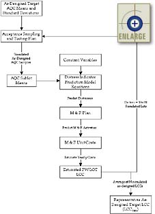Figure 7. Flow chart showing the process used to simulate the representative as-designed lot LCC (LCCDES).

Level 1 Pay Adjustments

Simulation of the Level 1 Individual AQC Pay Factor Curves

The data flow process used to compute the LCC for any one as-constructed lot is exactly the same as that used to compute the LCC for any one target as-designed simulated lot. As mentioned previously, the same constant variables, distress indicator models, acceptance sampling and testing plan, M & R plan, and cost models are used for both the as-designed and as-constructed lot simulations. The only difference between the procedures involves the AQC means and standard deviations used to define the quality of the as-designed and as-constructed pavement lots.

If a Level 1 pay adjustment approach is chosen, independent pay factor charts and corresponding equations are developed for each AQC. These pay factor charts are developed prior to the bidding on the project and are made available to the contractor. Hypothetical combinations of individual AQC means and standard deviations are selected and assumed to be equal to the as-constructed pavement lot quality. For each hypothetical combination, a representative as-constructed LCC is simulated using exactly the same procedure used for the simulation of the representative as-designed lot LCC (i.e., N AQC sample sets are simulated, resulting in N computed lot LCC's—the representative as-constructed lot LCC is computed as the mean of the N simulated as-constructed LCC values). Pay factors associated with each representative as-constructed LCC (hypothetical combination of AQC mean and standard deviation) are then determined using equation 3. (Note: Since these curves must be made available prior to accepting contractor bids, a representative bid price is used to compute the pay factors making up these curves [see the section titled Selecting an Appropriate Bid Price for Developing Level 1 Preconstruction Output in chapter 5, for more information]). Individual pay factor curves are constructed for specific levels of AQC standard deviation (chosen by the agency), and over a chosen range of AQC means, using the simulated representative as-constructed LCC's. Best-fit regression equations are then determined, representing the data making up the individual AQC pay factor curves. An example of a Level 1 pay factor chart for concrete strength is shown in figure 8.

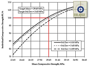Figure 8. Example of an individual Level 1 pay factor chart for concrete strength.

It is important to emphasize that only one AQC is allowed to vary at a time when developing these Level 1 AQC pay factor curves. For example, when representative pay factors are being simulated for the individual concrete strength pay factor chart, all simulated pay factors (from hypothetical combinations of concrete strength mean and standard deviation) are determined with the other AQC means and standard deviations (for slab thickness, air content, initial smoothness, and percent consolidation) set equal to their target values. Figure 9 contains a flow chart showing the general simulation process used to develop Level 1 AQC pay factor curves and corresponding pay factor regression equations. A more detailed step-by-step procedure for generating these Level 1 AQC pay factor curves and corresponding pay factor regression equations is presented in chapter 7.

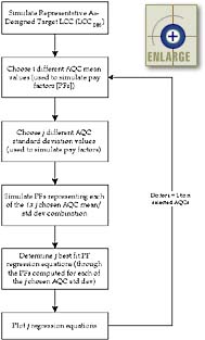Figure 9. Flow chart showing the process used to develop Level 1 AQC pay factor charts and corresponding equations.

Level 1 Composite Pay Factors

After the construction of an actual pavement lot, the agency takes samples from the pavement in accordance with the chosen acceptance sampling and testing plan. The AQC sampling and testing values measured in the field (for the given lot) are summarized into representative lot AQC means and standard deviations. The lot means and standard deviations are then used in the individual AQC pay factor regression equations to determine the corresponding independent AQC pay factors. The procedure used to determine individual AQC Level 1 pay factors from the pay factor charts is described in more detail in chapter 7.

Finally, the overall representative as-constructed Level 1 lot pay factor is determined by combining the individually calculated AQC pay factors into one CPF representing the lot. The CPF equation essentially provides the appropriate weighting factors for each independently determined AQC pay factor. This specific CPF function is determined by the agency. A more detailed discussion of the commonly used CPF equations is contained in chapter 6 in the section titled Defining a Level 1 Composite Pay Factor Equation. Figure 10 contains a flow chart showing the general process used to compute a Level 1 lot CPF.

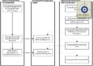Figure 10. Flow chart showing the process used to determine a Level 1 lot composite pay factor.

Level 2 Pay Adjustments

The Level 2 pay adjustment does not require the use of a CPF equation. The lot pay factor is directly computed through simulation with the PaveSpec 2.0 software. After the placement of the as-construction pavement lot, samples are taken from each sublot according to the agency-chosen acceptance sampling and testing plan. Each set of AQC sublot samples is then statistically summarized to obtain AQC means representing each sublot. The sublot means are used in the chosen distress indicators to predict sublot performance, predicted sublot M & R activities, and their associated sublot LCC's. Finally, these sublot LCC's are summarized into one representative lot present worth LCC. The overall as-constructed lot pay adjustment and pay factor are then determined using this calculated as-constructed lot LCC in equations 1 and 2, respectively. Figure 11 contains a flow chart showing the general simulation process used to calculate a Level 2 lot pay factor.

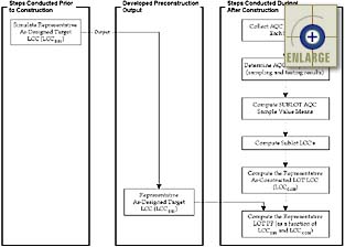Figure 11. Flow chart showing the process used to determine a Level 2 lot pay factor.

Major Differences Between Level 1 and Level 2 Pay Adjustment Procedures

Three of the primary differences between the Level 1 and 2 pay adjustment procedures include the following:

1. Preconstruction Output—Individual AQC pay factor curves are simulated using Level 1 procedures; the only Level 2 preconstruction output is the simulation of a representative as-designed LCC (LCC_DES).
   
   
2. Simulation of Pay Factors—Individual Level 1 AQC pay factor curves are simulated by holding all other AQC's at their target values; Level 2 pay factors allow for the simultaneous varying of all included AQC's (i.e., tradeoffs in AQC quality can occur).
   
   
3. Overall Lot Pay Factor Calculation Method—The overall Level 1 CPF is calculated as a function of the individually determined AQC pay factors computed using the simulated AQC pay factor charts and equations; the overall Level 2 pay factor is calculated directly using equation 3 in this volume. All required LCC's are determined using the PaveSpec 2.0 software.

It is important to emphasize that the Level 1 lot CPF is actually an estimate of the computed Level 2 lot pay factor. The Level 2 approach represents a simulated construction, sampling, testing, performance, and M & R over many years. Level 1 is a simplified method used to estimate the same pay factor as determined in Level 2, using more conventional pay factor curves.

Operating Characteristic Curves

Operating characteristic (OC) curves must be generated by the agency to determine if the chosen acceptance plan will perform as intended. The OC curves used with the PRS approach are similar to those used for conventional accept/reject acceptance plans, except that a set of OC curves is needed to reflect different payment options.⁽¹⁵⁾ An example of the OC curves, commonly constructed for adjustable payment acceptance plans using actual lot percent defective procedures, is illustrated in figure 12. Each set of OC curves is specific to a chosen sampling plan (i.e., number of sublots per lot, number of AQC samples per sublot, and types of AQC samples and tests). The development of these curves is an integral part of the specification development process in that they provide the agency and the contractor with information regarding their respective risk. Similar OC curves can be developed for Level 1 specifications using the PaveSpec 2.0 computer software. The OC curves developed under the PRS approach are plots of probability of acceptance at the pay level specified versus AQC mean (rather than percent defective). More detailed information regarding the development of these curves using PaveSpec 2.0 is contained in chapter 7 in the section titled Developing Operating Characteristic Curves.

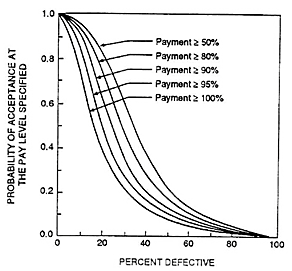Figure 12. Example of typical OC curves for an adjustable payment acceptance plan.(15)