3.0 Analysis Scenarios and ICM Strategies

This section describes the ICM strategies that will be applied to the Test Corridor and the scenarios that will be studied to analyze the impacts of the strategies. The objective of the Test Corridor modeling is to assess the practicality of the proposed AMS Framework. This section describes the strategies and scenarios for which the AMS modeling approach will be tested.

The ICM AMS framework provides tools and procedures capable of supporting the analysis of both recurrent and nonrecurrent corridor scenarios. Nonrecurrent congestion scenarios entail combinations of increases of demand and decreases of capacity. Figure 3.1 depicts how key ICM impacts may be lost if only “normal” travel conditions are considered; the proposed scenarios take into account both average- and high-travel demand, with and without incidents. The relative frequency of nonrecurrent conditions is important to estimate in this process – based on archived traffic conditions, as shown in Figure 3.2.

Figure 3.1 Key Intelligent Transportation System (ITS) Impacts May Be Lost If Only “Normal” Conditions Considered

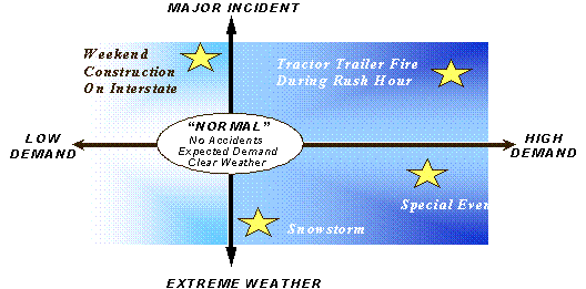
Source: Wunderlich, K., et al., Seattle 2020 Case Study, PRUEVIIN Methodology, Mitretek Systems. This document is available at the Federal Highway Administration Electronic Data Library (http://www.itsdocs.fhwa.dot.gov/).

Figure 3.2 Sources of System Variation – Classifying Frequency and Intensity

3.1 Average- and High-Demand Scenarios

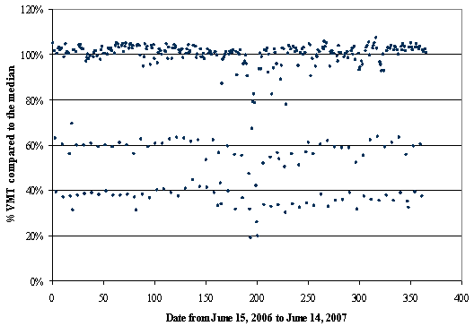
For the test corridor, average- and high-travel demand conditions were determined by analyzing archived data from the PeMS database. Table 3.1 shows average and maximum vehicle miles traveled (VMT) data for the entire region under Caltrans District 4. Typical weekday volumes for Tuesday, Wednesday, and Thursday show that maximum observed VMT is 6 percent higher than average VMT. Figure 3.3 provides an overview of demand patterns on the Test Corridor – the demand is lower on Saturday and Sunday, and during Christmas season. We chose to use “median” instead of “mean” demand to avoid bias from nonworking days.

Table 3.1 Determining High-Volume Scenario from VMT for Caltrans District 4

Day	Minimum	Mean	Maximum	Max/Mean	Max/Mean
Sunday	42,134,910	47,433,782	53,214,009	1.12	No value
Monday	42,251,727	55,616,955	60,296,132	1.08	No value
Tuesday	40,632,558	57,784,703	61,054,236	1.06	1.06
Wednesday	53,649,452	58,890,264	62,557,940	1.06	1.06
Thursday	46,971,959	59,607,667	63,807,090	1.07	1.06
Friday	50,495,376	61,664,122	65,244,922	1.06	No value
Saturday	48,530,858	53,343,231	58,004,132	1.09	No value

Figure 3.3 Demand Variation on the Test Corridor

Ranges of travel demand on the test corridor are as follows:

Low demand – Less than 98.5 percent of median VMT, or 42 percent of days in the year;
Medium demand – Between 98.5 percent and 102.5 percent of median VMT, or 29 percent of days in the year; and
High demand – Greater than 102.5 percent of median VMT, or 29 percent of days in the year.

The medians of the high and medium ranges will be used in the analysis. In the Test Corridor AMS we will simulate the median from the medium-demand range (100 percent) and the median from the high-demand range (104 percent). The average traffic volume scenario will be based on a trip table obtained for the AM peak period from the regional travel demand model.

3.2 Incident and No-Incident Scenarios

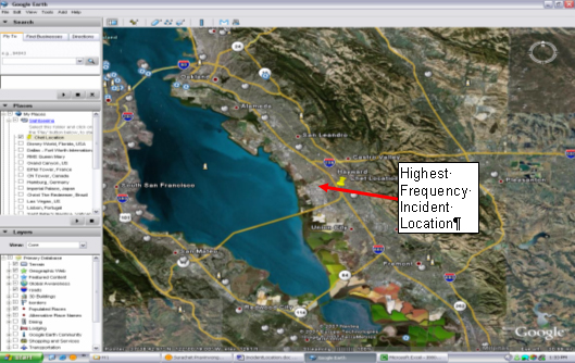
The most likely incident location for the Test Corridor was determined by analyzing incident frequency from the PeMS database. Figures 3.4 and 3.5 show incident locations by frequency on the Test Corridor, northbound and southbound, respectively. A plot of incident frequency on I‑880 southbound shows that the maximum number of incidents occur around Postmile 23, as shown in Figure 3.6. This location is shown in Figure 3.7 – between SR 23 and SR 92, an area of increased merging and weaving traffic.

Figure 3.4 Incident Locations/Frequency - Test Corridor NB

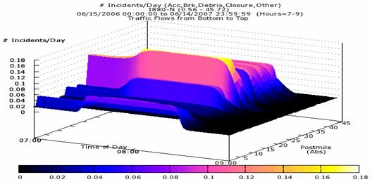
Figure 3.5 Incident Locations and Frequency on Test Corridor (Southbound)

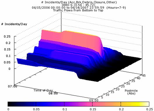
Figure 3.6 Incident Frequency in the Test Corridor (Southbound)

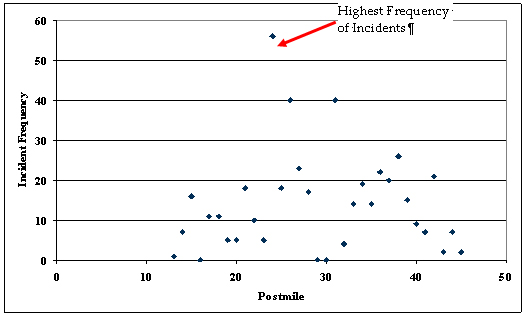
Figure 3.7 Highest Frequency Incident Location in the Test Corridor

Figure 3.7 is a satellite map indicating the location of the area with the highest frequency of incidents within the tested corridor.

The duration and severity of the incidents was obtained from a combination of the PeMS database and the “TMS Master Plan” study conducted for Caltrans. The PeMS graphic on incident duration is shown in Figure 3.8. Figure 3.9 shows incident duration by percent increments for incidents on the Test Corridor. We used aggregate incident data from June 15, 2006 to June 14, 2007 (including weekdays and weekends for all 365 days).

Figure 3.8 Incident Duration from PeMS

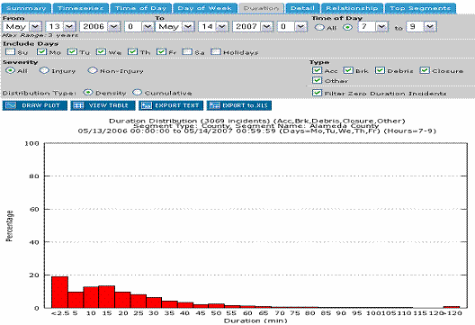
Figure 3.9 Incident Duration on the Test Corridor

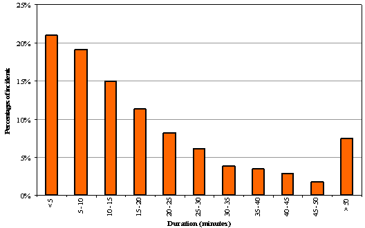
The nonrecurrent congestion (or incident) scenario includes an incident near Postmile 23 in the northbound direction. The incident will result in two lanes being closed for 45 minutes, starting at 7:15 a.m. This represents the 85th percentile incident with duration of 45 minutes. The Test Corridor at the incident location provides alternative arterial routes and alternative transportation modes, including bus and BART lines.

In addition to identifying high-incident locations and duration of incidents, when designing scenarios that describe operational conditions the analyst should also identify overall incident patterns as they occur on different days of the year. This type of analysis will be conducted in the Test Corridor AMS by separating major from minor incidents. Time and resource-permitting this analysis can be more thorough by focusing on different ranges of numbers of incidents occurring on different days of the year.

3.3 Summary of Analysis Settings

Table 3.2 presents a summary of settings for the Test Corridor analysis.

Table 3.2 Test Corridor – Summary of Analysis Settings

Parameter	Value	Comment
Analysis year	2005	The analysis year is based on the available model year in the regional travel demand model.
Time period of analysis	AM peak – 2 hours (7:00 a.m.-9:00 a.m.)	The analysis period is determined by the peak-hour trip table available in the regional travel demand model. The actual analysis period in the mesoscopic and microscopic simulation models will include an initialization period of 15 minutes and a demand dissipation period of 30 minutes.
Incident location	Postmile 23	Over 55 incidents have occurred around this postmile point between May 2006 and May 2007.
Incident duration	2 lanes closed for 45 minutes starting at 7:15	Obtained from incident duration from the PeMS database and Caltrans “TMS Master Plan” study.

Table 3.3 shows the overall frequency in operational conditions for the Test Corridor, including percentage of days in the year categorized by different incident and demand levels. Major incidents are defined as having duration over 20 minutes, and minor incidents as having duration under 20 minutes.

Table 3.3 Percentages of Days in the Year Categorized by Incident and Demand Levels

Demand	Incident Frequency: Minor Incident (Duration Less Than 20 Minutes)	Incident Frequency: Major Incident (Duration Greater Than 20 Minutes)	Total
High	20	9	29
Medium	21	8	29
Low	19	23	42
Total	61	39	100

3.4 ICM Strategies

The remainder of this section identifies site-specific strategies, analysis scenarios, and tools to be used in the analysis of implementation of integrated corridor management on the Test Corridor. This set of ICM strategies can comprehensively test the AMS methodology in terms of traveler responses (route diversion, mode shift, and temporal shift); and in terms of interfaces for flows of data between modeling tools. The Final Report will contain more detailed information on modeling of the Test Corridor. The subset of ICM strategies selected for testing includes the following:

Zero ITS baselines – Four combinations of average-/high-travel demand and presence (or not) of incident with no ITS (no ramp metering and no traveler information). The incident is defined as a two-lane blockage at the highest incident location for 45 minutes. The travel demand model and DynaSmart-P are used in modeling these scenarios.
Traveler information – Eight combinations of average-/high-travel demand and presence of incident with 1) pretrip traveler information, 2) en-route traveler information, 3) Variable Message Signs (VMS), and 4) combination of 1, 2, and 3. Traveler information on incident location and severity will provide drivers with the opportunity to take alternative arterial routes or drive to a transit station where parking is available. The analysis of these scenarios will be conducted in DynaSmart‑P.
Mode shift to transit in the presence of an incident – This scenario focuses on the evaluation of mode shift due to the incident. It will study the impact of parking availability by manipulating parking search time. Parking capacity at different BART stations will be taken into account. In this scenario, travel times from DynaSmart‑P will be imported in an external Geographic Information System (GIS)-based, mode-shift pivot point model. An iterative process will be applied to analyze mode choice for each 15-minute period.
Ramp metering – Freeway traffic management can be obtained by controlling the vehicles entering the freeway through ramp metering. The analysis of ramp metering will be conducted using DynaSmart‑P to assess regional diversion effects.
HOT lane – High-Occupancy Toll (HOT) lanes provide the potential to optimally use the HOV lanes while generating revenue. Converting the existing HOV lane in the I‑880 corridor will be studied using DynaSmart‑P. Mode shift effects will be studied using the pivot point mode shift model.
Arterial traffic signal coordination – Evaluation of arterial traffic signal coordination strategies using Synchro, DynaSmart-P, and the pivot-point mode choice model.
Combinations – Applying combinations of traveler information, transit, ramp metering, and HOT lane strategies will be evaluated. A combination of DynaSmart-P, and the pivot-point mode shift model will be used in this analysis.

The strategies and scenarios that will be studied on the Test Corridor are presented in Table 3.4.

Table 3.4 Test Corridor Analysis Scenarios

Scenario	Travel Demand	Incident	ICM Strategy	Description
Zero ITS baseline	Average, high	No, yes	No ITS	Combinations of average-/high-travel demand and presence (or not) of incident with no ITS (no ramp metering and no traveler information). Incident is defined as a 2-lane blockage at the highest incident location for 45 minutes.
ICM A	Average, high	Yes	Traveler information	DynaSmart-P and the pivot-point mode choice model – pretrip and en-route traveler information at 5% and 20% market penetration; VMS.
ICM B	Average, high	Yes	Mode shift to transit	Impact of incident information on mode shift will be studied using DynaSmart-P, the travel demand model, and the pivot-point mode choice model.
ICM C	Average, high	No, yes	Ramp metering	A ramp metering strategy will be studied using DynaSmart-P and the pivot-point mode choice model.
ICM D	Average, high	No, yes	HOT lane	Evaluation of HOT lane pricing will be studied using DynaSmart-P and the pivot-point mode choice model.
ICM E	Average, high	No, yes	Arterial traffic signal coordination	Evaluation of arterial traffic signal coordination strategies using Synchro, DynaSmart-P, and the pivot-point mode choice model.
ICM F	Average, high	No, yes	Combinations	Combinations of all ICM strategies will be studied using all available models

next | previous